统计机器学习Lecture-3
Lecturer: Prof.XIA
DONG
1. General linear regression
model.
 ## 1.1 general linear regression model - 内容:
general linear regression model.
## 1.1 general linear regression model - 内容:
general linear regression model.
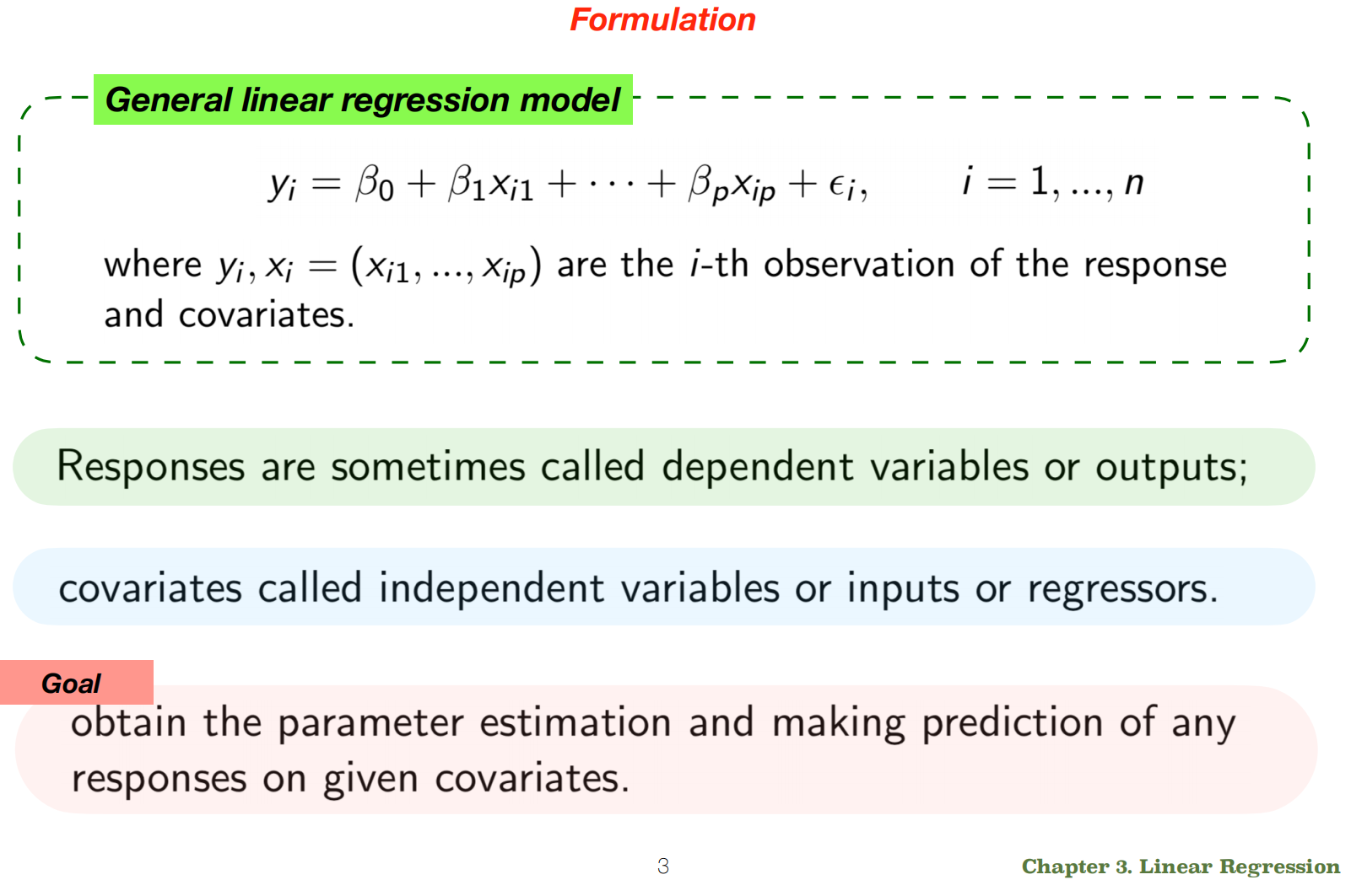
the fundamental equation:
\[y_i = \beta_0 + \beta_1x_{i1} + \dots +
\beta_px_{ip} + \epsilon_i\]
And it correctly identifies the main goal: to estimate the
parameters (the coefficients \(\beta_0, \beta_1, \dots, \beta_p\)) from
data so we can make predictions on new data.
核心目标:通过数据估计参数(即系数 \(\beta_0, \beta_1, \dots,
\beta_p\)),从而对新数据进行预测。
1.2
How we actually find the best values for the \(β\) coefficients (parameter
estimation)?:
- 内容: We find the best values for the \(\beta\) coefficients by finding the values
that minimize the overall error of the model. The most
common and fundamental method for this is called Ordinary Least
Squares (OLS).
##
The Main Method: Ordinary Least Squares (OLS) 普通最小二乘法 (OLS)
The core idea of OLS is to find the line (or hyperplane in multiple
dimensions) that is as close as possible to all the data points
simultaneously. OLS
的核心思想是找到一条尽可能同时接近所有数据点的直线(或多维超平面)。
1. Define the Error (Residuals)
误差
First, we need to define what “error” means. For any single data
point, the error is the difference between the actual value (\(y_i\)) and the value predicted by our model
(\(\hat{y}_i\)). This difference is
called the residual.
首先,需要定义“误差”的含义。对于任何单个数据点,误差是实际值 (\(y_i\)) 与模型预测值 (\(\hat{y}_i\))
之间的差值。这个差值称为残差。
Residual = Actual Value - Predicted Value
残差 = 实际值 - 预测值 \[e_i
= y_i - \hat{y}_i\]
You can visualize residuals as the vertical distance from each data
point to the regression line.
可以将残差可视化为每个数据点到回归线的垂直距离。
2.
The Cost Function: Sum of Squared Residuals 成本函数:残差平方和
We want to make all these residuals as small as possible. We can’t
just add them up, because some are positive and some are negative, and
they would cancel each other out.
所有残差尽可能小。不能简单地将它们相加,因为有些是正数,有些是负数,它们会相互抵消。
So, we square each residual (which makes them all positive) and then
sum them up. This gives us the Sum of Squared Residuals
(SSR), which is our “cost function.”
因此,将每个残差求平方(使它们都为正数),然后将它们相加。这就得到了残差平方和
(SSR),也就是“成本函数”。
\[SSR = \sum_{i=1}^{n} e_i^2 =
\sum_{i=1}^{n} (y_i - \hat{y}_i)^2\]
The goal of OLS is simple: find the values of \(\beta_0, \beta_1, \dots, \beta_p\) that
make this SSR value as small as possible.
3.
Solving for the Coefficients: The Normal Equation
求解系数:正态方程
For linear regression, calculus provides a direct, exact solution to
this minimization problem. By taking the derivative of the SSR function
with respect to each \(\beta\)
coefficient and setting it to zero, we can solve for the optimal values.
对于线性回归,微积分为这个最小化问题提供了直接、精确的解。通过对 SSR
函数的每个 \(\beta\)
系数求导并将其设为零,就可以求解出最优值。
This process results in a formula known as the Normal
Equation, which can be expressed cleanly using matrix algebra:
这个过程会得到一个称为正态方程的公式,它可以用矩阵代数清晰地表示出来:
\[\hat{\boldsymbol{\beta}} =
(\mathbf{X}^T\mathbf{X})^{-1}\mathbf{X}^T\mathbf{y}\]
- \(\hat{\boldsymbol{\beta}}\) is the
vector of our estimated coefficients.估计系数的向量。
- \(\mathbf{X}\) is a matrix where
each row is an observation and each column is a feature (with an added
column of 1s for the intercept \(\beta_0\)).其中每一行代表一个观测值,每一列代表一个特征(截距
\(\beta_0\) 增加了一列全为 1
的值)。
- \(\mathbf{y}\) is the vector of the
actual response values.实际响应值的向量。
Statistical software and programming libraries (like Scikit-learn in
Python) use this equation (or more computationally stable versions of
it) to find the best coefficients for you instantly.
## An
Alternative Method: Gradient Descent 梯度下降
While the Normal Equation gives a direct answer, it can be very slow
if you have a massive number of features (e.g., hundreds of thousands).
An alternative, iterative method used across machine learning is
Gradient Descent.
The Intuition: Imagine the SSR cost function is a
big valley. Your initial (random) \(\beta\) coefficients place you somewhere on
the slope of this valley.
- Check the slope (the gradient) at your current
position. 检查您当前位置的斜率(梯度)。
- Take a small step in the steepest downhill
direction. 朝最陡的下坡方向迈出一小步**。
- Repeat. You keep taking steps downhill until you
reach the bottom of the valley. The bottom of the valley represents the
minimum SSR, and your coordinates at that point are the optimal \(\beta\) coefficients.
重复。您继续向下走,直到到达山谷底部。谷底代表最小SSR,该点的坐标即为最优\(\beta\)系数。
The size of each “step” you take is controlled by a parameter called
the learning rate. Gradient Descent is the foundational
optimization algorithm for many complex models, including neural
networks.
每次“步进”的大小由一个称为学习率的参数控制。梯度下降是许多复杂模型(包括神经网络)的基础优化算法。
## Summary: OLS vs. Gradient
Descent
| Feature |
Ordinary Least Squares (OLS) |
Gradient Descent |
| How it works |
Direct calculation using the Normal
Equation. |
Iterative; takes steps to minimize
error. |
| Pros |
Provides an exact, optimal solution. No
parameters to tune. |
More efficient for very large datasets.
Very versatile. |
| Cons |
Can be computationally expensive with many
features. |
Requires choosing a learning rate. May not
find the exact minimum. |
2. Simple Linear Regression
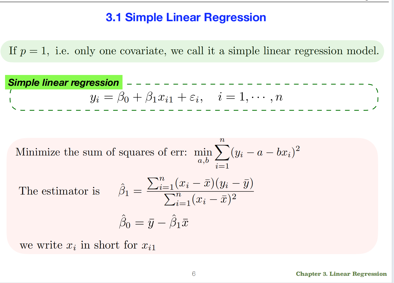
2.1 Simple Linear Regression
- 内容: Simple Linear Regression: a
special case of the general model you showed earlier where you only have
one predictor variable (\(p=1\)).
## The Model and the Goal
模型和目标
Sets up the simplified equation for a line: \[y_i = \beta_0 + \beta_1x_i + \epsilon_i\]
* \(y_i\) is the outcome you want to
predict.要预测的结果。 * \(x_i\) is
your single input feature or covariate.单个输入特征或协变量。 * \(\beta_1\) is the slope of
the line. It tells you how much \(y\)
is expected to increase for a one-unit increase in \(x\).表示 \(x\) 每增加一个单位,\(y\) 预计会增加多少。 * \(\beta_0\) is the
intercept. It’s the predicted value of \(y\) when \(x\) is zero.当 \(x\) 为零时 \(y\) 的预测值。 * \(\epsilon_i\) is the random error
term.是随机误差项。
The goal, stated as “Minimize the sum of squares of err,” is exactly
the Ordinary Least Squares (OLS) method we just
discussed. It’s written here as: \[\min_{a,b}
\sum_{i=1}^{n} (y_i - a - bx_i)^2\] This is just a different way
of writing the same thing, where they use a for the
intercept (\(\beta_0\)) and
b for the slope (\(\beta_1\)). You’re trying to find the
specific values of the slope and intercept that make the sum of all the
squared errors as small as possible.
目标,即“最小化误差平方和”,正是普通最小二乘法
(OLS)。: \[\min_{a,b}
\sum_{i=1}^{n} (y_i - a - bx_i)^2\] 这是另一种写法,其中用
a 表示截距 (\(\beta_0\)),b 表示斜率 (\(\beta_1\))。尝试找到斜率和截距的具体值,使得所有平方误差之和尽可能小。
The most important part of this slide is the
solution. For the simple case with only one variable,
you don’t need complex matrix algebra (the Normal Equation). Instead,
the minimization problem can be solved with these two straightforward
formulas:
对于只有一个变量的简单情况,不需要复杂的矩阵代数(正态方程)。相反,最小化问题可以用以下两个简单的公式来解决:
1. The Slope: \(\hat{\beta}_1\)
\[\hat{\beta}_1 = \frac{\sum_{i=1}^{n}
(x_i - \bar{x})(y_i - \bar{y})}{\sum_{i=1}^{n} (x_i -
\bar{x})^2}\] * Intuition: This formula might
look complex, but it’s actually very intuitive. * The numerator, \(\sum(x_i - \bar{x})(y_i - \bar{y})\), is
closely related to the covariance between X and Y. It
measures whether X and Y tend to move in the same direction (positive
slope) or in opposite directions (negative slope). 与 X 和 Y
之间的协方差密切相关。它衡量 X 和 Y
是倾向于朝相同方向(正斜率)还是朝相反方向(负斜率)移动。 * The
denominator, \(\sum(x_i - \bar{x})^2\),
is related to the variance of X. It measures how much X
varies on its own. 它衡量 X 自身的变化量。 * In short, the slope
is a measure of how X and Y vary together, scaled by how much X varies
by itself. 斜率衡量的是 X 和 Y 共同变化的程度,并以 X
自身的变化量为标度。
2. The Intercept: \(\hat{\beta}_0\) 截距
\[\hat{\beta}_0 = \bar{y} -
\hat{\beta}_1\bar{x}\] * Intuition: This formula
is even simpler and has a wonderful geometric meaning. It ensures that
the line of best fit always passes through the “center of mass”
of the data, which is the point of averages \((\bar{x}, \bar{y})\).
它确保最佳拟合线始终穿过数据的“质心”,即平均值 \((\bar{x}, \bar{y})\) 的点。计算出最佳斜率
(\(\hat{\beta}_1\))
后,就可以将其代入此公式。然后,可以调整截距 (\(\hat{\beta}_0\)),使直线完美地围绕数据云的中心点旋转。
* Once you’ve calculated the best slope (\(\hat{\beta}_1\)), you can plug it into this
formula. You then adjust the intercept (\(\hat{\beta}_0\)) so that the line pivots
perfectly around the central point of your data cloud.
In summary, this slide provides the precise, closed-form formulas to
calculate the slope and intercept for the line of best fit in a simple
linear regression model.
3. Statistical Inference
 ## 3.1 Statistical Inference - 内容:
Statistical Inference: These two slides are deeply
connected and explain how we go from just calculating the
coefficients to understanding how accurate and
reliable they are.
解释了我们如何从仅仅计算系数到理解它们的准确性和可靠性。
## 3.1 Statistical Inference - 内容:
Statistical Inference: These two slides are deeply
connected and explain how we go from just calculating the
coefficients to understanding how accurate and
reliable they are.
解释了我们如何从仅仅计算系数到理解它们的准确性和可靠性。
## The
Core Problem: Quantifying Uncertainty 量化不确定性
The second slide poses the fundamental questions: * “How accurate are
\(\hat{\beta}_0\) and \(\hat{\beta}_1\)?”准确性如何? * “What are
the distributions of \(\hat{\beta}_0\)
and \(\hat{\beta}_1\)?”分布是什么?
The reason we ask this is that our estimated coefficients (\(\hat{\beta}_0, \hat{\beta}_1\)) were
calculated from a specific sample of data. If we
collected a different random sample from the same population, we would
get slightly different estimates.估计的系数 (\(\hat{\beta}_0, \hat{\beta}_1\))
是根据特定的数据样本计算出来的。如果我们从同一总体中随机抽取不同的样本,我们得到的估计值会略有不同。
The goal of statistical inference is to use the estimates from our
single sample to make conclusions about the true, unknown
population parameters (\(\beta_0,
\beta_1\)) and to quantify our uncertainty about
them.统计推断的目标是利用单个样本的估计值得出关于真实、未知的总体参数(\(\beta_0,
\beta_1\))的结论,并量化对这些参数的不确定性。
##
The Key Assumption That Makes It Possible 实现这一目标的关键假设
To figure out the distribution of our estimates, we must make an
assumption about the distribution of the errors. This is the most
important assumption in linear regression for inference:
为了确定估计值的分布,必须对误差的分布做出假设。这是线性回归推断中最重要的假设:
Assumption: \(\epsilon_i
\stackrel{\text{i.i.d.}}{\sim} N(0, \sigma^2)\)
This means we assume the random error terms are: * Normally
distributed (\(N\)).*
正态分布(\(N\))。 *
Have a mean of zero (our model is correct on average).*
均值为零(模型平均而言是正确的)。 * Have a constant
variance \(\sigma^2\)
(homoscedasticity).* 方差为常数\(\sigma^2\)(方差齐性)。 * Are
independent and identically distributed (i.i.d.),
meaning each error is independent of the others.*
是独立同分布(i.i.d.)的,这意味着每个误差都独立于其他误差。
Why is this important? Because our coefficients
\(\hat{\beta}_0\) and \(\hat{\beta}_1\) are calculated as weighted
sums of the \(y_i\) values, and the
\(y_i\) values depend on the errors
\(\epsilon_i\). This assumption about
the errors allows us to prove that our estimated coefficients themselves
are also normally distributed. 系数 \(\hat{\beta}_0\) 和 \(\hat{\beta}_1\) 是通过 \(y_i\) 值的加权和计算的,而 \(y_i\) 值取决于误差 \(\epsilon_i\)。这个关于误差的假设使能够证明估计的系数本身也服从正态分布。
##
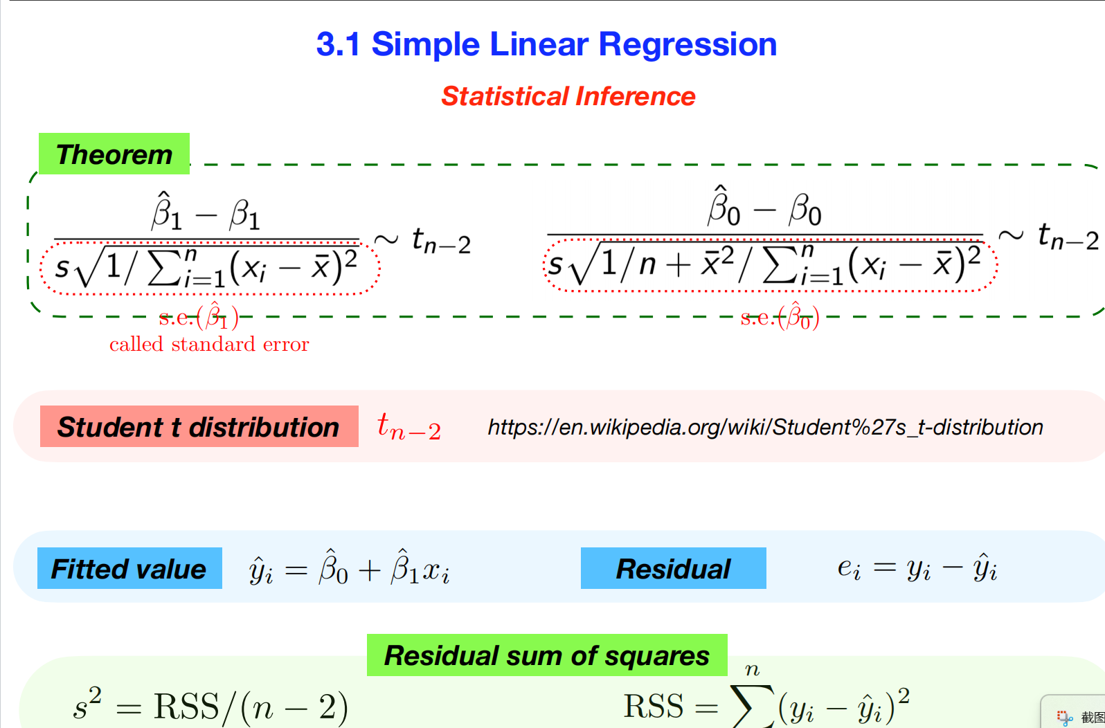
The Solution: The Theorem and the t-distribution 定理和 t 分布
The first slide provides the central theorem that allows us to
perform inference. It tells us exactly how to standardize our estimated
coefficients so they follow a known distribution.
第一张幻灯片提供了进行推断的核心定理。它准确地告诉我们如何对估计的系数进行标准化,使其服从已知的分布。
1. The Standard Error
(s.e.) 标准误差 (s.e.)
First, look at the denominators in the red dotted boxes. These are
the standard errors of the coefficients,
s.e.($\hat{\beta}_1$) and
s.e.($\hat{\beta}_0$).
第一张幻灯片提供了进行推断的核心定理。它准确地告诉我们如何对估计的系数进行标准化,使其服从已知的分布。
- What it is: The standard error is the estimated
standard deviation of the coefficient’s sampling
distribution. In simpler terms, it’s a measure of the average
amount by which our estimate \(\hat{\beta}_1\) would differ from the true
\(\beta_1\) if we were to repeat the
experiment many times.
标准误差是系数抽样分布的标准差估计值。简单来说,它衡量的是如果我们重复实验多次,我们估计的
\(\hat{\beta}_1\) 与真实的 \(\beta_1\) 之间的平均差异。
- A smaller standard error means a more precise and reliable
estimate.
标准误差越小,估计值越精确可靠。
2. The t-statistic t 统计量
The theorem shows two fractions that form a
t-statistic. The general structure for this is:
该定理展示了两个构成t 统计量的分数。其一般结构如下:
\[t = \frac{\text{ (Sample Estimate - True
Value) }}{\text{ Standard Error of the Estimate }}\]
For \(\beta_1\), this is: \(\frac{\hat{\beta}_1 -
\beta_1}{\text{s.e.}(\hat{\beta}_1)}\).
The key insight is that this specific quantity follows a
Student’s t-distribution with \(n-2\) degrees of freedom.
关键在于,这个特定量服从学生 t
分布,其自由度为\(n-2\)。 * Student’s
t-distribution:** This is a probability distribution that looks very
similar to the normal distribution but has slightly “heavier” tails. We
use it instead of the normal distribution because we had to
estimate the standard deviation of the errors (s
in the formula), which adds extra uncertainty.
这是一种概率分布,与正态分布非常相似,但尾部略重。使用它来代替正态分布,是因为必须估计误差的标准差(公式中的
s),这会增加额外的不确定性。 * Degrees of Freedom
(n-2): We start with n data points, but we lose
two degrees of freedom because we used the data to estimate two
parameters: \(\beta_0\) and \(\beta_1\). 从 n
个数据点开始,但由于用这些数据估计了两个参数:\(\beta_0\) 和 \(\beta_1\),因此损失了两个自由度。 #### 3.
Estimating the Error Variance (\(s^2\))估计误差方差 (\(s^2\)) To calculate the standard errors, we
need a value for s, which is our estimate of the true error
standard deviation \(\sigma\). This is
calculated from the Residual Sum of Squares (RSS).
为了计算标准误差,我们需要一个 s 的值,它是对真实误差标准差
\(\sigma\)
的估计值。该值由残差平方和 (RSS) 计算得出。 *
RSS: First, we calculate the RSS = \(\sum(y_i - \hat{y}_i)^2\), which is the sum
of all the squared errors.* RSS:首先,计算 RSS = \(\sum(y_i -
\hat{y}_i)^2\),即所有平方误差之和。 * \(s^2\): Then, we find the estimate
of the error variance: \(s^2 = \text{RSS} /
(n-2)\). We divide by \(n-2\) to
get an unbiased estimate. * \(s^2\):然后,计算误差方差的估计值:\(s^2 = \text{RSS} / (n-2)\)。我们将其除以
\(n-2\) 即可得到无偏估计值。 *
s is simply the square root of \(s^2\). This s is the value
used in the standard error formulas.* s 就是 \(s^2\) 的平方根。这个 s
是标准误差公式中使用的值。
## What This Allows
Us To Do (The Practical Use)
Because we know the exact distribution of our t-statistic, we can now
achieve our goal of quantifying uncertainty: 因为知道 t
统计量的精确分布,所以现在可以实现量化不确定性的目标:
- Hypothesis Testing: We can test if a predictor is
actually useful. The most common test is for the null hypothesis \(H_0: \beta_1 = 0\). If we can prove the
observed \(\hat{\beta}_1\) is very
unlikely to occur if the true \(\beta_1\) were zero, we can conclude there
is a statistically significant relationship between \(x\) and \(y\).
可以检验一个预测变量是否真的有用。最常见的检验是零假设 \(H_0: \beta_1 = 0\)。如果能证明,当真实的
\(\beta_1\) 为零时,观测到的 \(\hat{\beta}_1\)
不太可能发生,那么就可以得出结论,\(x\)
和 \(y\)
之间存在统计学上的显著关系。
- Confidence Intervals: We can construct a range of
plausible values for the true coefficient. For example, we can calculate
a 95% confidence interval for \(\beta_1\). This gives us a range where we
are 95% confident the true value of \(\beta_1\) lies.
可以为真实系数构建一系列合理的值。
4. Multiple Linear Regression
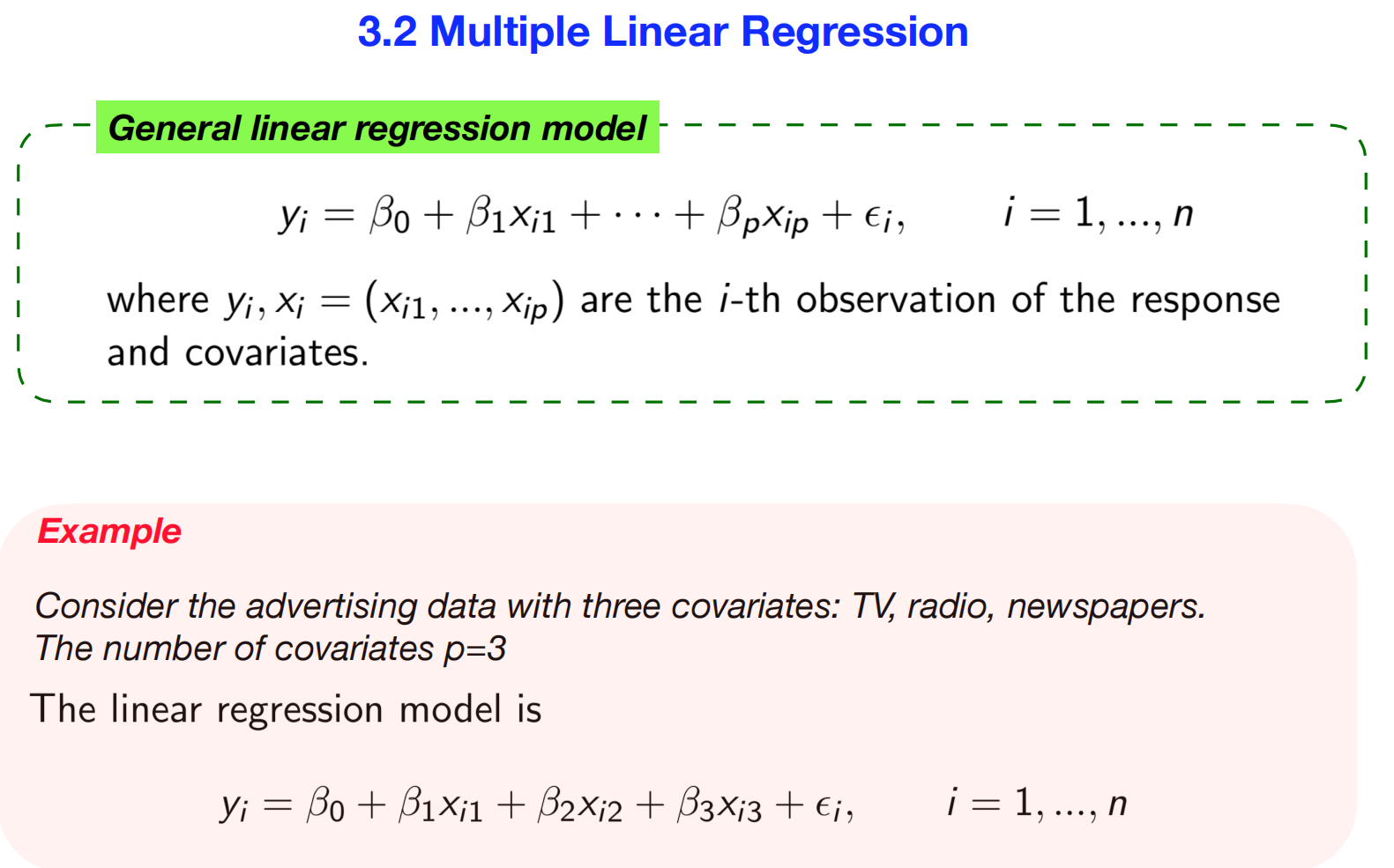
 ## 4.1 Multiple Linear Regression - 内容:
Multiple Linear Regression:
## 4.1 Multiple Linear Regression - 内容:
Multiple Linear Regression:
Here’s a detailed breakdown that connects both slides.
##
The Model: From One to Many Predictors 从单预测变量到多预测变量
The first slide introduces the Multiple Linear Regression
model. This is a direct extension of the simple model, but
instead of using just one predictor variable, we use multiple (\(p\)) predictors to explain our response
variable.
多元线性回归模型是简单模型的直接扩展,但不是只使用一个预测变量,而是使用多个(\(p\))预测变量来解释响应变量。
The general formula is: \[y_i = \beta_0 +
\beta_1x_{i1} + \beta_2x_{i2} + \dots + \beta_px_{ip} +
\epsilon_i\]
Key Change in Interpretation
This is the most important new concept. In simple regression, \(\beta_1\) was just the slope. In multiple
regression, each coefficient has a more nuanced meaning:
在简单回归中,\(\beta_1\)
只是斜率。在多元回归中,每个系数都有更微妙的含义:
\(\beta_j\) is the average
change in \(y\) for a one-unit increase
in \(x_j\), while holding all other
predictors constant.
This is incredibly powerful. Using the advertising example from your
slide: * \(y_i = \beta_0 +
\beta_1(\text{TV}_i) + \beta_2(\text{Radio}_i) +
\beta_3(\text{Newspaper}_i) + \epsilon_i\) * \(\beta_1\) represents the effect of TV
advertising on sales, after controlling for the amount
spent on Radio and Newspaper ads. This allows you to isolate the unique
contribution of each advertising
channel.表示在控制广播和报纸广告支出后,电视广告对销售额的影响。这可以让您区分每个广告渠道的独特贡献。
## The
Solution: Deriving the Normal Equation 推导正态方程
The second slide shows the mathematical process for finding the best
coefficients (\(\beta_0, \beta_1, \dots,
\beta_p\)) using the Ordinary Least Squares
(OLS) method. It’s essentially a condensed derivation of the
Normal Equation. 使用普通最小二乘法
(OLS) 寻找最佳系数 (\(\beta_0,
\beta_1, \dots, \beta_p\))
的数学过程。它本质上是正态方程的简化推导。
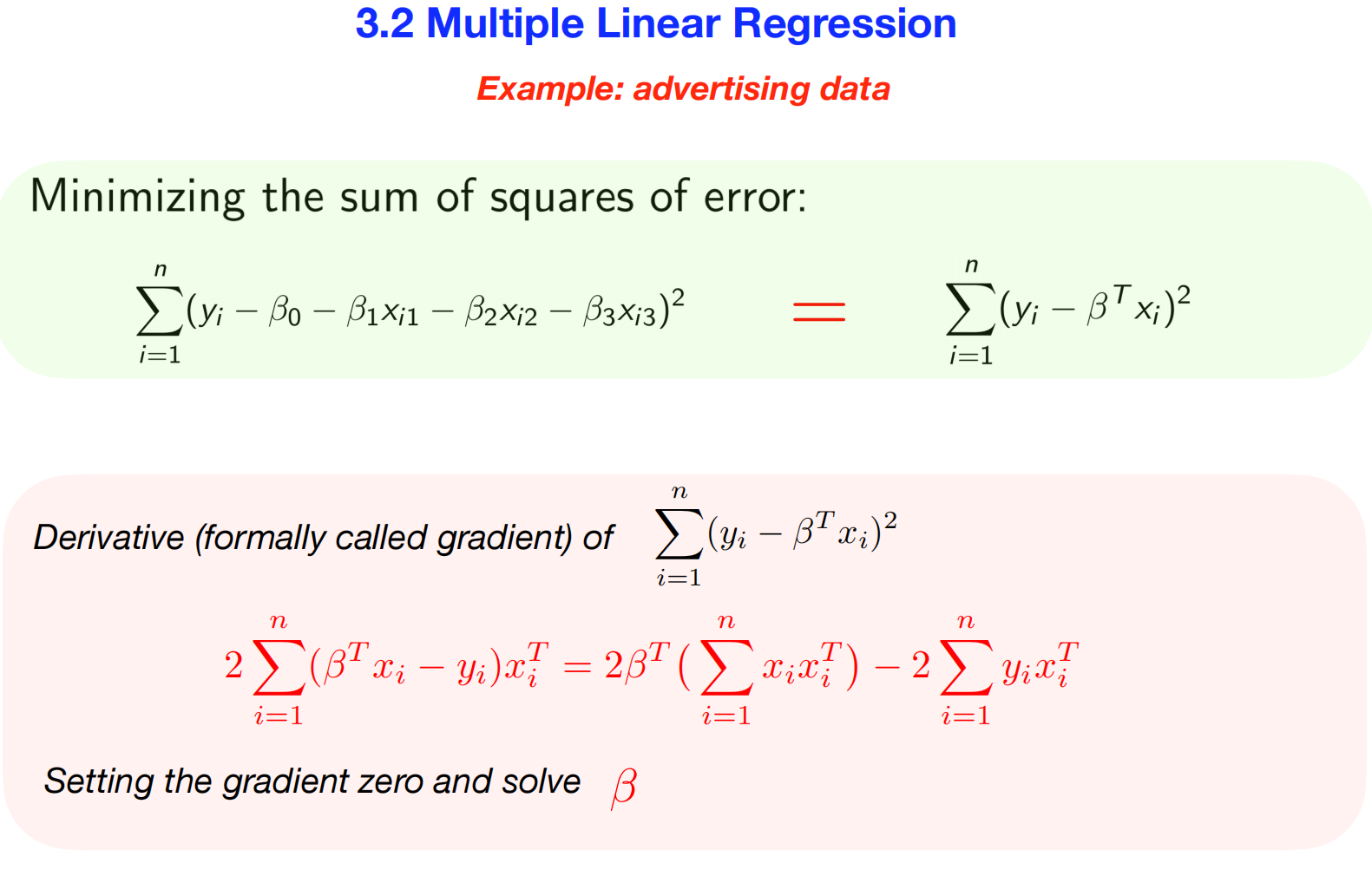
1. The
Goal: Minimizing the Sum of Squares 最小化平方和
Just like before, our goal is to minimize the sum of the squared
errors (or residuals): 目标是最小化平方误差(或残差)之和。
- Scalar Form: \(\sum_{i=1}^{n} (y_i - \beta_0 - \beta_1x_{i1} -
\beta_2x_{i2} - \beta_3x_{i3})^2\)
- This is easy to read but gets very long with more variables.
代码易于阅读,但变量越多,代码越长。
- Vector Form: \(\sum_{i=1}^{n} (y_i - \boldsymbol{\beta}^T
\mathbf{x}_i)^2\)
- This is a more compact and powerful way to write the same thing
using linear algebra, where \(\boldsymbol{\beta}^T \mathbf{x}_i\) is the
dot product that calculates the entire predicted value \(\hat{y}_i\).
这是一种更简洁、更强大的线性代数表示方法,其中 \(\boldsymbol{\beta}^T \mathbf{x}_i\)
是计算整个预测值 \(\hat{y}_i\)
的点积。
2.
The Method: Using Calculus to Find the Minimum 使用微积分求最小值
To find the set of \(\beta\) values
that results in the lowest possible error, we use calculus.
The Derivative (Gradient): Since our error
function depends on multiple \(\beta\)
coefficients, we can’t take a simple derivative. Instead, we take the
gradient, which is a vector of partial derivatives (one
for each coefficient). This tells us the “slope” of the error function
in every direction. 导数(梯度) 误差函数依赖于多个 \(\beta\)
系数,因此我们不能简单地求导数。相反,采用梯度,它是一个由偏导数组成的向量(每个系数对应一个偏导数)。这告诉误差函数在各个方向上的“斜率”。
Setting the Gradient to Zero: The minimum of a
function occurs where its slope is zero (the very bottom of the error
“valley”). The slide shows the result of taking this gradient and
setting it to
zero.函数的最小值出现在其斜率为零的地方(即误差“谷底”的最低点)。幻灯片展示了取此梯度并将其设为零的结果。
The equation shown on the slide: \[2
\sum_{i=1}^{n} (\boldsymbol{\beta}^T \mathbf{x}_i - y_i)\mathbf{x}_i^T =
0\] …is the result of this calculus step. The goal is now to
algebraically rearrange this equation to solve for \(\boldsymbol{\beta}\).
是这一微积分步骤的结果。现在的目标是用代数方法重新排列这个方程,以求解
\(\boldsymbol{\beta}\)。
3. The Result: The
Normal Equation 正则方程
After rearranging the equation from the previous step and expressing
the sums in their full matrix form, we arrive at a clean and beautiful
solution. While the slide doesn’t show the final step, the result of
“Setting the gradient zero and solve \(\beta\)” is the Normal
Equation:
重新排列上一步中的方程,并将和表示为完整的矩阵形式后,得到了一个简洁美观的解。虽然幻灯片没有展示最后一步,“设置梯度零点并求解
\(\beta\)”
的结果就是正态方程:
\[\hat{\boldsymbol{\beta}} =
(\mathbf{X}^T\mathbf{X})^{-1}\mathbf{X}^T\mathbf{y}\]
- \(\hat{\boldsymbol{\beta}}\) is the
vector of our optimal coefficient estimates.
- \(\mathbf{X}\) is the “design
matrix” where each row is an observation and each column is a predictor
variable. \(\mathbf{X}\)
是“设计矩阵”,其中每一行代表一个观测值,每一列代表一个预测变量。
- \(\mathbf{y}\) is the vector of our
response variable. \(\mathbf{y}\)
是我们的响应变量的向量。
This single equation is the general solution for finding the OLS
coefficients for any linear regression model, no matter
how many predictors you have. This is what statistical software
calculates for you under the hood.
无论有多少个预测变量,这个简单的方程都是任何线性回归模型中
OLS 系数的通解。
5. matrix notatio
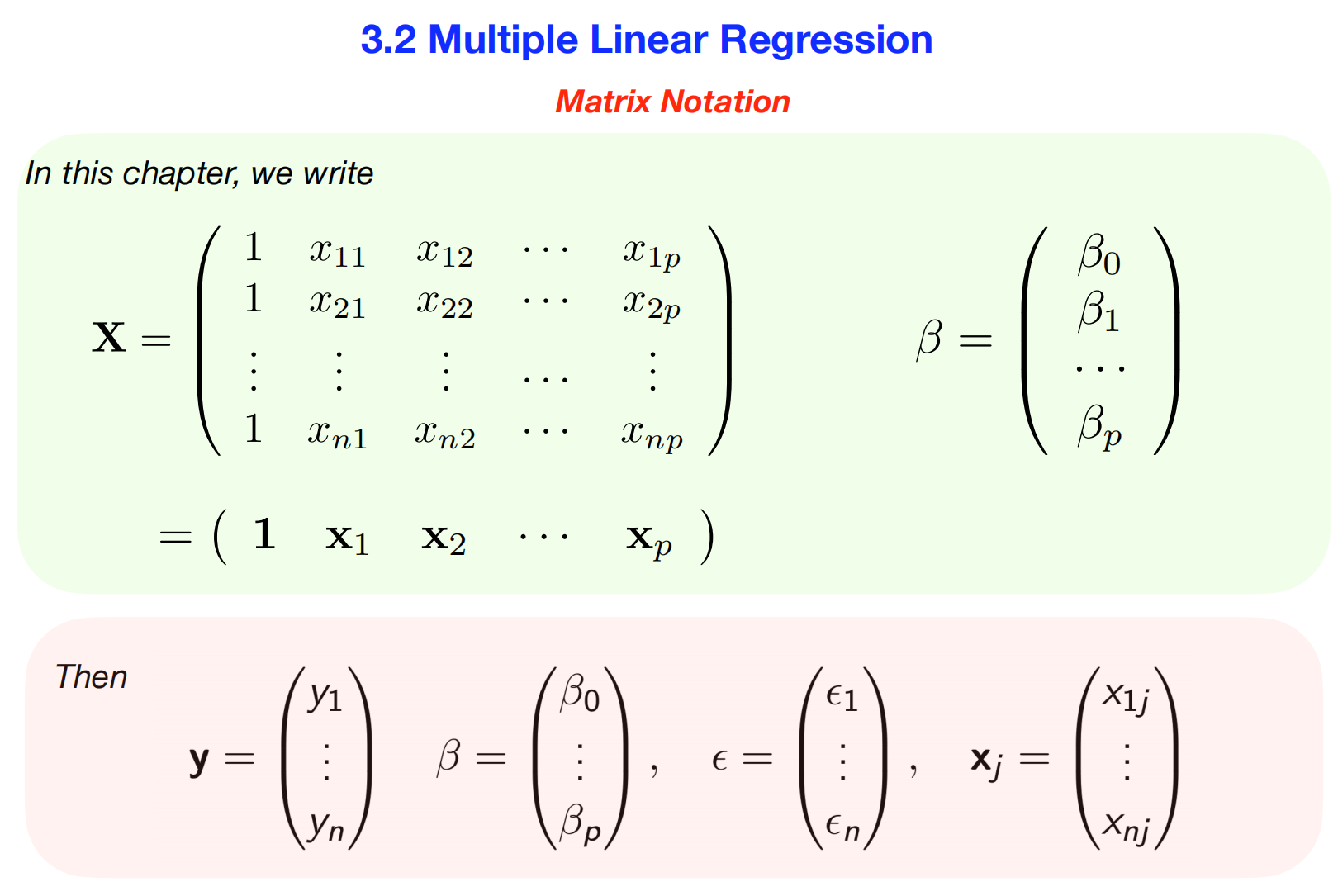
- 内容: This slide introduces the matrix
notation for multiple linear regression, which is a powerful
way to represent the entire system of equations in a compact form. This
notation isn’t just for tidiness—it’s the foundation for how the
solutions are derived and calculated in software.
多元线性回归的矩阵符号,这是一种以紧凑形式表示整个方程组的有效方法。这种符号不仅仅是为了简洁,它还是软件中推导和计算解的基础。
Here is a more detailed breakdown.
## Why Use Matrix Notation?
Imagine you have 10,000 observations (\(n=10,000\)) and 5 predictor variables
(\(p=5\)). Writing out the model
equation for each observation would be impossible: \(y_1 = \beta_0 + \beta_1x_{11} + \dots +
\beta_5x_{15} + \epsilon_1\) \(y_2 =
\beta_0 + \beta_1x_{21} + \dots + \beta_5x_{25} + \epsilon_2\)
…and so on for 10,000 lines.
假设你有 10,000 个观测值(n=10,000)和 5
个预测变量(p=5)。为每个观测值写出模型方程是不可能的: \(y_1 = \beta_0 + \beta_1x_{11} + \dots +
\beta_5x_{15} + \epsilon_1\) \(y_2 =
\beta_0 + \beta_1x_{21} + \dots + \beta_5x_{25} + \epsilon_2\)
……以此类推,直到 10,000 行。 Matrix notation allows us to consolidate
this entire system into a single, elegant
equation:矩阵符号使我们能够将整个系统合并成一个简洁的方程: \[\mathbf{y} = \mathbf{X}\boldsymbol{\beta} +
\boldsymbol{\epsilon}\] Let’s break down each component shown on
your slide.
## The Components Explained
1. The Design Matrix: \(\mathbf{X}\) 设计矩阵
\[\mathbf{X} = \begin{pmatrix} 1 &
x_{11} & x_{12} & \cdots & x_{1p} \\ 1 & x_{21} &
x_{22} & \cdots & x_{2p} \\ \vdots & \vdots & \vdots
& \ddots & \vdots \\ 1 & x_{n1} & x_{n2} & \cdots
& x_{np} \end{pmatrix}\] This is the most important matrix.
It contains all of your predictor variable
data.这是最重要的矩阵。它包含所有预测变量数据。 * Rows:
Each row represents a single observation (e.g., a person, a company, a
day). There are n
rows.每一行代表一个观察值(例如,一个人、一家公司、一天)。共有
n 行。 * Columns: Each column
represents a predictor variable. There are p predictor
columns, plus one special column.每列代表一个预测变量。共有
p 个预测列,外加一个特殊列。 * The Column of
Ones: This is a crucial detail. This first column of all ones
is a placeholder for the intercept term (\(\beta_0\)). When you perform
matrix multiplication, this 1 gets multiplied by \(\beta_0\), ensuring the intercept is
included in the model for every single observation.
这是一个至关重要的细节。第一列(全 1)是截距项 (\(\beta_0\))
的占位符。执行矩阵乘法时,这个 1 会乘以 \(\beta_0\),以确保截距包含在模型中,适用于每个观测值。
2. The
Coefficient Vector: \(\boldsymbol{\beta}\) 系数向量
\[\boldsymbol{\beta} = \begin{pmatrix}
\beta_0 \\ \beta_1 \\ \vdots \\ \beta_p \end{pmatrix}\] This is a
column vector that contains all the model parameters—the unknown values
we want to estimate. The goal of linear regression is to find the
numerical values for this vector.
3. The Response Vector:
\(\mathbf{y}\) 响应向量
\[\mathbf{y} = \begin{pmatrix} y_1 \\
\vdots \\ y_n \end{pmatrix}\] This is a column vector containing
all the observed outcomes you are trying to predict (e.g., sales, test
scores, stock prices).
4. The Error
Vector: \(\boldsymbol{\epsilon}\)
误差向量
\[\boldsymbol{\epsilon} = \begin{pmatrix}
\epsilon_1 \\ \vdots \\ \epsilon_n \end{pmatrix}\] This column
vector bundles together all the individual, unobserved random errors. It
represents the portion of y that our model cannot
explain with X.
## Putting It All Together
When you write the equation \(\mathbf{y} =
\mathbf{X}\boldsymbol{\beta} + \boldsymbol{\epsilon}\), you are
actually representing the entire system of individual equations.
Let’s look at the multiplication \(\mathbf{X}\boldsymbol{\beta}\): \[\begin{pmatrix} 1 & x_{11} & \dots &
x_{1p} \\ 1 & x_{21} & \dots & x_{2p} \\ \vdots & \vdots
& \ddots & \vdots \\ 1 & x_{n1} & \dots & x_{np}
\end{pmatrix} \begin{pmatrix} \beta_0 \\ \beta_1 \\ \vdots \\ \beta_p
\end{pmatrix} = \begin{pmatrix} 1\cdot\beta_0 + x_{11}\cdot\beta_1 +
\dots + x_{1p}\cdot\beta_p \\ 1\cdot\beta_0 + x_{21}\cdot\beta_1 + \dots
+ x_{2p}\cdot\beta_p \\ \vdots \\ 1\cdot\beta_0 + x_{n1}\cdot\beta_1 +
\dots + x_{np}\cdot\beta_p \end{pmatrix}\] As you can see, the
result of this multiplication is a single column vector where each row
is the “predictor” part of the regression equation for that observation.
此乘法的结果是一个单列向量,其中每一行都是该观测值的回归方程的“预测变量”部分。
By setting this equal to \(\mathbf{y} -
\boldsymbol{\epsilon}\), you perfectly recreate the entire set of
n equations in one clean statement. This compact form is
what allows us to easily derive and compute the Normal
Equation solution: \(\hat{\boldsymbol{\beta}} =
(\mathbf{X}^T\mathbf{X})^{-1}\mathbf{X}^T\mathbf{y}\).这种紧凑形式使我们能够轻松推导和计算正态方程的解
6.
the core mathematical conclusion of Ordinary Least Squares (OLS)
- 内容: Of course. These slides present the core
mathematical conclusion of Ordinary Least Squares (OLS) and a key
geometric property that explains why this solution works.
展示了普通最小二乘法 (OLS)
的核心数学结论,以及一个关键的几何性质,解释了该解决方案为何有效。
Let’s break down the concepts and the calculation processes in
detail.
##
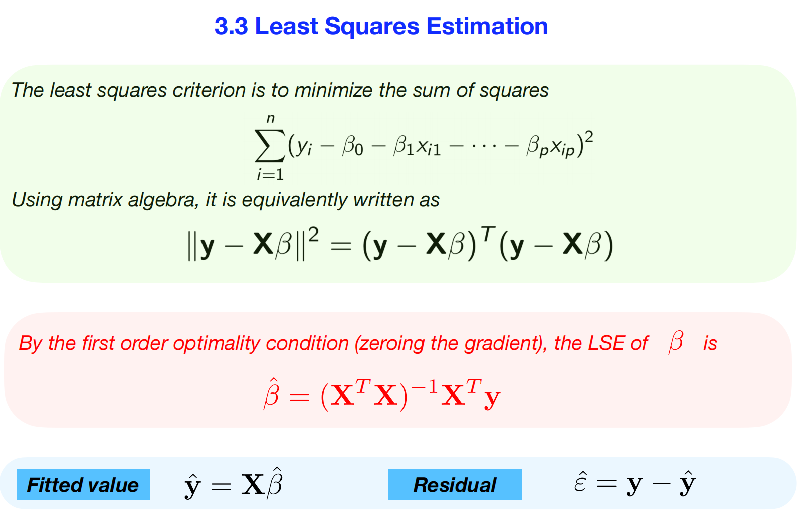
Part 1: The Objective and the Solution (Slide 1) 最小化几何距离
This slide summarizes the entire OLS problem and its solution in the
language of matrix algebra.
The Concept:
Minimizing Geometric Distance
“最小二乘准则”是我们模型的目标。 The “least squares criterion” is the
objective of our model. The slide shows it in two equivalent forms:
- Summation Form: \(\sum_{i=1}^{n} (y_i - \beta_0 - \beta_1x_{i1} -
\dots - \beta_px_{ip})^2\) This is the sum of the squared
differences between the actual values (\(y_i\)) and the predicted values. 这是实际值
(\(y_i\)) 与预测值之差的平方和。
- Matrix Form: \(||\mathbf{y} - \mathbf{X}\boldsymbol{\beta}||^2 =
(\mathbf{y} - \mathbf{X}\boldsymbol{\beta})^T(\mathbf{y} -
\mathbf{X}\boldsymbol{\beta})\) This is the more powerful way to
view the problem. Think of \(\mathbf{y}\) (the vector of all actual
outcomes) and \(\mathbf{X}\boldsymbol{\beta}\) (the vector
of all predicted outcomes) as two points in an n-dimensional space. The
expression \(||\mathbf{y} -
\mathbf{X}\boldsymbol{\beta}||^2\) represents the squared
Euclidean distance between these two points. 将 \(\mathbf{y}\)(所有实际结果的向量)和 \(\mathbf{X}\boldsymbol{\beta}\)(所有预测结果的向量)视为
n 维空间中的两个点。表达式 \(||\mathbf{y} -
\mathbf{X}\boldsymbol{\beta}||^2\)
表示这两点之间的平方欧氏距离。 Therefore, the OLS
problem is a geometric one: Find the coefficient vector \(\boldsymbol{\beta}\) that makes the
predicted values vector \(\mathbf{X}\boldsymbol{\beta}\) as close as
possible to the actual values vector \(\mathbf{y}\). 因此,OLS
问题是一个几何问题:找到一个系数向量 \(\boldsymbol{\beta}\),使预测值向量 \(\mathbf{X}\boldsymbol{\beta}\)
尽可能接近实际值向量 \(\mathbf{y}\)。
The
Solution: The Least Squares Estimator (LSE)最小二乘估计器
(LSE)
The slide provides the direct solution to this minimization problem,
which is the Normal
Equation:此最小化问题的直接解,即正态方程:
\[\hat{\boldsymbol{\beta}} =
(\mathbf{X}^T\mathbf{X})^{-1}\mathbf{X}^T\mathbf{y}\]
This formula gives you the exact vector of coefficients \(\hat{\boldsymbol{\beta}}\) that minimizes
the squared distance. We get this formula by taking the gradient (the
multidimensional version of a derivative) of the distance function with
respect to \(\boldsymbol{\beta}\),
setting it to zero, and solving, as hinted at in your previous slides.
给出了使平方距离最小化的精确系数向量 通过取距离函数关于 \(\boldsymbol{\beta}\)
的梯度(导数的多维版本),将其设为零,然后求解,即可得到此公式。
Finally, the slide defines: * Fitted values: \(\hat{\mathbf{y}} =
\mathbf{X}\hat{\boldsymbol{\beta}}\) (The vector of predictions
using our optimal coefficients). 拟合值 * Residuals:
\(\hat{\boldsymbol{\epsilon}} = \mathbf{y} -
\hat{\mathbf{y}}\) (The vector of errors, representing the
difference between actuals and
predictions).误差向量,表示实际值与预测值之间的差异
##
Part 2: The Geometric Property and Proofs (Slide 2)几何性质及证明
This slide explains a beautiful and fundamental property of the least
squares solution:
orthogonality.解释了最小二乘解的一个美妙而基本的性质:正交性。
The
Concept: Orthogonality of Residuals残差的正交性
The main idea is that the residual vector \(\hat{\boldsymbol{\epsilon}}\) is
orthogonal (perpendicular) to every predictor variable
in your model. 主要思想是残差向量 \(\hat{\boldsymbol{\epsilon}}\)
与模型中的每个预测变量正交(垂直)。
Geometric Intuition: Think of the columns of
your matrix \(\mathbf{X}\) (i.e., your
predictors and the intercept) as defining a flat surface, or a
“hyperplane,” in a high-dimensional space. Your actual data vector \(\mathbf{y}\) exists somewhere in this
space, likely not on the hyperplane. The OLS process finds the point on
that hyperplane, \(\hat{\mathbf{y}}\),
that is closest to \(\mathbf{y}\). The
shortest line from a point to a plane is always one that is
perpendicular to the plane. The residual vector, \(\hat{\boldsymbol{\epsilon}} = \mathbf{y} -
\hat{\mathbf{y}}\), is that line. 将矩阵 \(\mathbf{X}\)
的列(即预测变量和截距)想象成在高维空间中定义一个平面或“超平面”。实际数据向量
\(\mathbf{y}\)
存在于该空间的某个位置,可能不在超平面上。OLS 过程会在该超平面 \(\hat{\mathbf{y}}\) 上找到与 \(\mathbf{y}\)
最接近的点。从一个点到一个平面的最短线始终是与该平面垂直的线。残差向量
\(\hat{\boldsymbol{\epsilon}} = \mathbf{y} -
\hat{\mathbf{y}}\) 就是这条直线。
Mathematical Statement: This geometric property
is stated as \(\mathbf{X}^T
\hat{\boldsymbol{\epsilon}} = \mathbf{0}\). This equation means
that the dot product of the residual vector with every column of \(\mathbf{X}\) is zero, which is the
mathematical definition of orthogonality. 该等式意味着残差向量与 \(\mathbf{X}\)
每一列的点积都为零,这正是正交性的数学定义。
The Calculation
Process (The Proofs)
1. Proof of Orthogonality: The slide shows a
step-by-step calculation to prove that \(\mathbf{X}^T \hat{\boldsymbol{\epsilon}}\)
is indeed zero. * Step 1: Start with the expression to
be proven: \(\mathbf{X}^T
\hat{\boldsymbol{\epsilon}}\) 从待证明的表达式开始: *
Step 2: Substitute the definition of the residual,
\(\hat{\boldsymbol{\epsilon}} = \mathbf{y} -
\mathbf{X}\hat{\boldsymbol{\beta}}\): \[\mathbf{X}^T (\mathbf{y} -
\mathbf{X}\hat{\boldsymbol{\beta}})\] 代入残差的定义 *
Step 3: Distribute the \(\mathbf{X}^T\): \[\mathbf{X}^T \mathbf{y} -
\mathbf{X}^T\mathbf{X}\hat{\boldsymbol{\beta}}\]分配
Step 4: Substitute the Normal Equation for \(\hat{\boldsymbol{\beta}}\): \[\mathbf{X}^T \mathbf{y} - \mathbf{X}^T\mathbf{X}
[(\mathbf{X}^T\mathbf{X})^{-1}\mathbf{X}^T\mathbf{y}]\] *
Step 5: The key step is the cancellation. A matrix
\((\mathbf{X}^T\mathbf{X})\) multiplied
by its inverse \((\mathbf{X}^T\mathbf{X})^{-1}\) equals the
identity matrix \(\mathbf{I}\), which
acts like the number 1 in multiplication. \[\mathbf{X}^T \mathbf{y} - \mathbf{I}
\mathbf{X}^T\mathbf{y} = \mathbf{X}^T \mathbf{y} -
\mathbf{X}^T\mathbf{y} = \mathbf{0}\] 关键步骤是消去。 This
completes the proof, showing that the orthogonality property is a direct
consequence of the Normal Equation solution.
2. Proof of LSE: This is a more abstract proof
showing that our \(\hat{\boldsymbol{\beta}}\) truly gives the
minimum possible error. It uses the orthogonality property and the
Pythagorean theorem for vectors. It essentially shows that for any other
possible coefficient vector \(\boldsymbol{v}\), the error \(||\mathbf{y} -
\mathbf{X}\boldsymbol{v}||^2\) will always be greater than or
equal to the error from our LSE, \(||\mathbf{y} -
\mathbf{X}\hat{\boldsymbol{\beta}}||^2\).
7.geometric interpretation
These two slides together provide a powerful geometric interpretation
of how Ordinary Least Squares (OLS) works, centered on the concepts of
orthogonality and projection.
以正交性和投影的概念为中心,从几何角度有力地诠释了普通最小二乘法
(OLS) 的工作原理。
Here’s a detailed summary of the concepts and the processes they
describe.
## Summary
These slides explain that the process of finding the “best fit” line
in regression is geometrically equivalent to projecting
the actual data vector (\(\mathbf{y}\))
onto a hyperplane defined by the predictor variables (\(\mathbf{X}\)). This projection splits the
actual data into two perpendicular components:
解释了回归分析中寻找“最佳拟合”直线的过程,其几何意义等同于将实际数据向量
(\(\mathbf{y}\))
投影到由预测变量 (\(\mathbf{X}\))
定义的超平面上。此投影将实际数据拆分为两个垂直分量:
- The Fitted Values (\(\hat{\mathbf{y}}\)): The part of
the data that is perfectly explained by the model (the projection).
数据中能够被模型完美解释的部分(投影)。
- The Residuals (\(\hat{\boldsymbol{\epsilon}}\)):
The part of the data that is unexplained (the error), which is
perpendicular to the explained part.
数据中无法解释的部分(误差),它与被解释部分垂直。 A special tool called
the projection matrix (H), or “hat matrix,” is
introduced as the operator that performs this projection.
引入一个称为投影矩阵
(H)(或称“帽子矩阵”)的特殊工具,作为执行此投影的运算符。
## Concepts and
Process Explained in Detail
1.
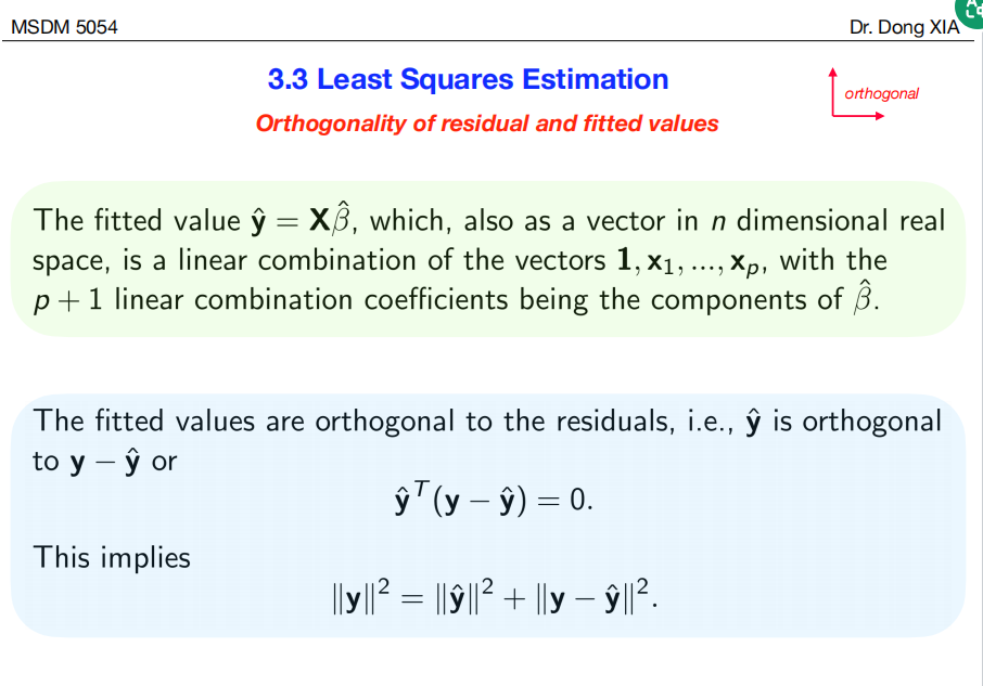
The Fitted Values as a Linear Combination 拟合值作为线性组合
The first slide starts by stating that the fitted value vector \(\hat{\mathbf{y}} =
\mathbf{X}\hat{\boldsymbol{\beta}}\) is a linear
combination of the columns of \(\mathbf{X}\) (your predictors).
Concept: This means that the vector of fitted
values, \(\hat{\mathbf{y}}\), must lie
within the geometric space (a line, plane, or hyperplane) spanned by
your predictor variables. The model is incapable of producing a
prediction that does not live in this space. 这意味着拟合值向量 \(\hat{\mathbf{y}}\)
必须位于预测变量所构成的几何空间(直线、平面或超平面)内。模型无法生成不存在于此空间的预测。
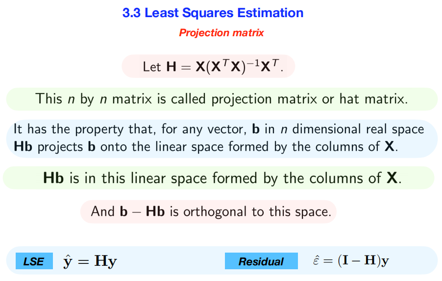
#### 2. The Projection Matrix (The “Hat Matrix”) 投影矩阵(“帽子矩阵”)
The second slide introduces the tool that makes this projection happen:
the projection matrix, also called the hat
matrix, H.
Definition: \(\mathbf{H} =
\mathbf{X}(\mathbf{X}^T\mathbf{X})^{-1}\mathbf{X}^T\)
Process: This matrix has a special job. When you
multiply it by any vector (like our data vector \(\mathbf{y}\)), it projects that vector onto
the space spanned by the columns of \(\mathbf{X}\). We can see this by starting
with our definition of fitted values and substituting the normal
equation solution for \(\hat{\boldsymbol{\beta}}\): \[\hat{\mathbf{y}} =
\mathbf{X}\hat{\boldsymbol{\beta}} =
\mathbf{X}[(\mathbf{X}^T\mathbf{X})^{-1}\mathbf{X}^T\mathbf{y}] =
[\mathbf{X}(\mathbf{X}^T\mathbf{X})^{-1}\mathbf{X}^T]\mathbf{y}\]
This shows that: \[\hat{\mathbf{y}} =
\mathbf{H}\mathbf{y}\] This is why H is
nicknamed the hat matrix—it “puts the hat” on \(\mathbf{y}\).
这个矩阵有其特殊的用途。当你将它乘以任何向量(例如我们的数据向量 \(\mathbf{y}\))时,它会将该向量投影到由
\(\mathbf{X}\) 的列所跨越的空间上。
#### 3. The Orthogonality of Fitted Values and Residuals
拟合值和残差的正交性 This is the central concept of the first slide and
a fundamental property of least squares.
Concept: The fitted value vector (\(\hat{\mathbf{y}}\)) and the residual vector
(\(\hat{\boldsymbol{\epsilon}} = \mathbf{y} -
\hat{\mathbf{y}}\)) are orthogonal
(perpendicular) to each other.
Mathematical Statement: Their dot product is
zero: \(\hat{\mathbf{y}}^T(\mathbf{y} -
\hat{\mathbf{y}}) = 0\).
Geometric Intuition: This means the vectors
\(\mathbf{y}\), \(\hat{\mathbf{y}}\), and \(\hat{\boldsymbol{\epsilon}}\) form a
right-angled triangle in n-dimensional space. The
actual data vector \(\mathbf{y}\) is
the hypotenuse, while the model’s prediction \(\hat{\mathbf{y}}\) and the error \(\hat{\boldsymbol{\epsilon}}\) are the two
perpendicular legs. 这意味着向量 \(\mathbf{y}\)、\(\hat{\mathbf{y}}\) 和 \(\hat{\boldsymbol{\epsilon}}\) 在 n
维空间中构成一个直角三角形。实际数据向量 \(\mathbf{y}\) 是斜边,而模型的预测值 \(\hat{\mathbf{y}}\) 和误差值 \(\hat{\boldsymbol{\epsilon}}\)
是两条垂直边。
4. The Pythagorean
Theorem of Least Squares
The orthogonality relationship directly implies the Pythagorean
theorem.
- Formula: \(||\mathbf{y}||^2 = ||\hat{\mathbf{y}}||^2 +
||\mathbf{y} - \hat{\mathbf{y}}||^2\)
- Concept: This is one of the most important
equations in statistics, as it partitions the total variance in the
data. 这是统计学中最重要的方程之一,因为它可以分割数据中的总方差。
- \(||\mathbf{y}||^2\) is
proportional to the Total Sum of Squares (TSS): The
total variation of the response variable around its
mean.响应变量围绕其均值的总变异。
- \(||\hat{\mathbf{y}}||^2\) is
proportional to the Explained Sum of Squares (ESS): The
portion of the total variation that is explained by your regression
model.回归模型可以解释的总变异部分。
- \(||\mathbf{y} -
\hat{\mathbf{y}}||^2\) is the Residual Sum of Squares
(RSS): The portion of the total variation that is left
unexplained (the error).总变异中未解释的部分(即误差)。
This relationship, Total Variation = Explained Variation +
Unexplained Variation, is the foundation for calculating
metrics like R-squared (\(R^2\)), which measures the
goodness of fit of your model. 总变异 = 解释变异 +
未解释变异,是计算R 平方 (\(R^2\))
等指标的基础,该指标用于衡量模型的拟合优度。
5. Residuals
and the Identity Matrix 残差和单位矩阵
Finally, the second slide shows that just as H
projects onto the “model space,” a related matrix projects onto the
“error space.” 最后,第二张幻灯片显示,正如H
投影到“模型空间”一样,相关矩阵也会投影到“误差空间”。 *
Process: We can express the residuals using the hat
matrix: \[\hat{\boldsymbol{\epsilon}} =
\mathbf{y} - \hat{\mathbf{y}} = \mathbf{y} - \mathbf{H}\mathbf{y} =
(\mathbf{I} - \mathbf{H})\mathbf{y}\] The matrix \((\mathbf{I} - \mathbf{H})\) is also a
projection matrix. It takes the original data vector \(\mathbf{y}\) and projects it onto the space
that is orthogonal to all of your predictors, giving you the residual
vector directly.
8.visualization
of Ordinary Least Squares (OLS) regression
_regression.png)
This slide provides an excellent geometric visualization of what’s
happening “under the hood” in Ordinary Least Squares (OLS) regression.
It translates the algebraic formulas into a more intuitive spatial
concept. 这张幻灯片以出色的几何可视化方式展现了普通最小二乘 (OLS)
回归的“幕后”机制。它将代数公式转化为更直观的空间概念。
## Summary
The image shows that the process of finding the least squares
estimates is geometrically equivalent to taking the actual
outcome vector (\(\mathbf{y}\)) and finding its
orthogonal projection (\(\hat{\mathbf{y}}\)) onto a
hyperplane formed by the predictor variables (\(\mathbf{x}_1\) and \(\mathbf{x}_2\)). The projection \(\hat{\mathbf{y}}\) is the vector of fitted
values, representing the closest possible approximation of the real data
that the model can achieve.
该图显示,寻找最小二乘估计值的过程在几何上等同于将实际结果向量
(\(\mathbf{y}\))
求出其正交投影 (\(\hat{\mathbf{y}}\)) 到由预测变量 (\(\mathbf{x}_1\) 和 \(\mathbf{x}_2\)
构成的超平面上。投影 \(\hat{\mathbf{y}}\)
是拟合值的向量,表示模型能够达到的与真实数据最接近的近似值。
## The Concepts
Explained Spatially空间概念解释
Let’s break down each element of the diagram and its meaning:
1. The Space Itself 空间本身
- Concept: We are not in a simple 2D or 3D graph
where axes are X and Y. Instead, we are in an n-dimensional
space, where n is the number of observations
in your dataset. Each axis in this space corresponds to one observation
(e.g., one person, one day).
我们并非身处一个简单的二维或三维图形中,其中坐标轴为 X 和
Y。相反,我们身处一个 n 维空间,其中 n
是数据集中的观测值数量。此空间中的每个轴对应一个观测值(例如,一个人,一天)。
- Meaning: A vector like y or
x₁ is a single point in this high-dimensional space.
For example, if you have 50 data points, y is a vector
pointing to a specific location in a 50-dimensional space. 像
y 或 x₁
这样的向量是这个高维空间中的单个点。例如,如果您有 50
个数据点,y 就是指向 50 维空间中特定位置的向量。
2.
The Predictor Hyperplane (The Yellow
Surface)预测变量超平面(黄色表面)
- Concept: The vectors for your predictor variables,
x₁ and x₂, define a flat surface. If
you had only one predictor, this would be a line. With two, it’s a
plane. With more, it’s a hyperplane.预测变量的向量
x₁ 和 x₂
定义了一个平面。如果只有一个预测变量,它就是一条线。如果有两个,它就是一个平面。如果有更多的预测变量,它就是一个超平面。
- Meaning: This yellow plane represents the
“world of possible predictions” that your model is
allowed to make. Any linear combination of your predictors—which is what
a linear regression model calculates—will result in a vector that lies
somewhere on this surface.
这个黄色平面代表你的模型可以做出的“可能预测的世界”。任何预测变量的线性组合(也就是线性回归模型计算的结果)都会产生一个位于这个平面某处的向量。
#### 3. The Actual Outcome Vector (y)实际结果向量 (y)
- Concept: The red vector y
represents your actual, observed data. It’s a single point in the
n-dimensional space. 红色向量 y
代表你实际观察到的数据。它是 n 维空间中的一个点。
- Meaning: Critically, this vector usually does
not lie on the predictor hyperplane. If it did, your
model would be a perfect fit with zero error. The fact that it’s “off
the plane” represents the real-world noise and variation that the model
cannot fully capture.
至关重要的是,这个向量通常不位于预测变量超平面上。如果它位于超平面上,你的模型将完美拟合,误差为零。它“偏离平面”代表了模型无法完全捕捉到的真实世界的噪声和变化。
4. The Fitted Value
Vector (ŷ)拟合值向量 (ŷ)
- Concept: Since y is not on the
plane, we find the point on the plane that is geometrically
closest to y. This closest point is found by
dropping a perpendicular line from y to the plane. The
point where it lands is the orthogonal projection,
labeled ŷ (y-hat). 由于 y
不在平面上,因此我们在平面上找到与 y
几何上最接近的点。这个最接近点是通过从 y**
到平面做一条垂直线找到的。垂直线所在的点就是正交投影,标记为
ŷ (y-hat)。
- Meaning: ŷ is the vector of your model’s
fitted values. It is the “best” possible approximation of the
real data that can be created using the given predictors because it
minimizes the distance (and therefore the squared error) between the
actual data (y) and the model’s prediction. ŷ
是模型拟合值的向量。它是使用给定预测变量可以创建的对真实数据的“最佳”近似值,因为它最小化了实际数据
(y)
与模型预测值之间的距离(从而最小化了平方误差)。
5. The Residual
Vector (The Dashed Line)残差向量(虚线)
- Concept: The dashed line connecting the tip of
y to the tip of ŷ is the
residual vector (\(\boldsymbol{\epsilon} = \mathbf{y} -
\hat{\mathbf{y}}\)). Its length is the shortest possible distance
from y to the hyperplane.
连接y顶点和ŷ顶点的虚线是残差向量
(\(\boldsymbol{\epsilon} = \mathbf{y} -
\hat{\mathbf{y}}\))。其长度是从y到超平面的最短可能距离。
- Meaning: This vector represents the
error of the model—the part of the actual data that is
left over after accounting for the predictors. The right-angle symbol
(└) is the most important part of the diagram, as it shows this error is
orthogonal (perpendicular) to the prediction and to all
the predictors. This visualizes the core property that the model’s
errors are uncorrelated with the predictors.
连接y顶点和ŷ顶点的虚线是残差向量
(\(\boldsymbol{\epsilon} = \mathbf{y} -
\hat{\mathbf{y}}\))。其长度是从y到超平面的最短可能距离。
9.Singular
Value Decomposition (SVD) 奇异值分解 (SVD)
These slides delve into the more advanced linear algebra behind the
projection matrix (H), explaining its fundamental
properties and offering a new way to construct it using Singular
Value Decomposition (SVD). 探讨了投影矩阵 (H)
背后更高级的线性代数,解释了它的基本性质,并提供了一种使用奇异值分解
(SVD) 构造它的新方法。
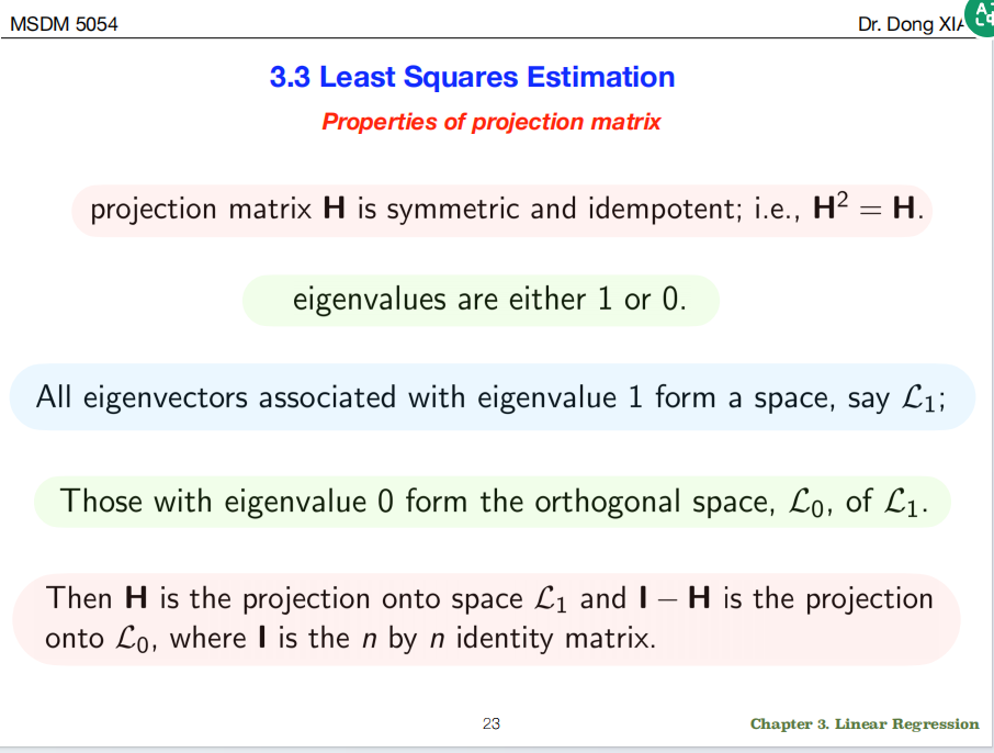
## Summary
These slides show that the projection matrix (H),
which is central to least squares, has two key mathematical properties:
it’s symmetric and idempotent
(projecting twice is the same as projecting once). These properties
dictate that its eigenvalues must be either 1 or 0. Singular Value
Decomposition (SVD) of the data matrix X provides an
elegant and numerically stable way to express H as
UUᵀ, which makes these fundamental properties easier to
understand and prove. 这些幻灯片展示了投影矩阵
(H)(最小二乘法的核心)的两个关键数学性质:对称和幂等(投影两次等于投影一次)。这些性质决定了它的特征值必须为
1 或 0。数据矩阵 X 的奇异值分解 (SVD)
提供了一种优雅且数值稳定的方式,将H 表示为
UUᵀ,这使得这些基本性质更容易理解和证明。
## Concepts and
Process Explained in Detail
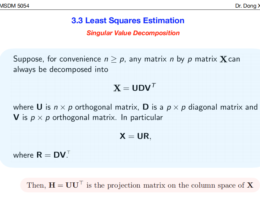
1. Singular Value
Decomposition (SVD)
The first slide introduces SVD, a powerful method for factoring any
matrix.
- Concept: SVD breaks down your data matrix
X into three simpler matrices: X =
UDVᵀ. Think of this as revealing the fundamental structure of
your data.SVD 将数据矩阵 X
分解为三个更简单的矩阵:X =
UDVᵀ。这可以理解为揭示数据的基本结构。
- U: An orthogonal matrix whose
columns form a perfect, orthonormal basis for the space spanned by your
predictors (the column space of X). These columns
represent the principal directions of your data’s
space.一个正交矩阵,其列构成预测变量所占空间(X
的列空间)的完美正交基。这些列代表数据空间的主方向。
- D: A diagonal matrix containing
the “singular values,” which measure the importance or magnitude of each
of these principal
directions.一个对角矩阵,包含“奇异值”,用于衡量每个主方向的重要性或大小。
- V: Another orthogonal
matrix.另一个正交矩阵。
- Process (How SVD simplifies the Projection Matrix) SVD
如何简化投影矩阵: The main takeaway from this slide is the new,
simpler formula for the hat matrix: \[\mathbf{H} = \mathbf{UU}^T\] This result
is derived by substituting X = UDVᵀ into the original,
more complex formula for H: \[\mathbf{H} =
\mathbf{X}(\mathbf{X}^T\mathbf{X})^{-1}\mathbf{X}^T\] When you
perform this substitution and use the fact that for orthogonal matrices
U and V, we have UᵀU =
I and VᵀV = I, the D and
V matrices completely cancel out, leaving the
beautifully simple form H = UUᵀ. This tells us that
projection is fundamentally about the basis vectors (U)
of the predictor space. 执行此代入并利用正交矩阵 U 和
V 的公式,即 UᵀU = I 和 VᵀV =
I,D 和 V
矩阵完全抵消,剩下简洁的形式 H =
UUᵀ。这告诉我们,投影本质上是关于预测空间的基向量(U)的。
2.
The Properties of the Projection Matrix (H) 投影矩阵 (H) 的性质
The second slide describes the essential nature of any projection
matrix.
Symmetric (H = Hᵀ): This property ensures that
the projection is orthogonal (i.e., it finds the closest point by moving
perpendicularly).
此性质确保投影是正交的(即,它通过垂直移动找到最近的点)。
Idempotent (H² = H): This is the most intuitive
property of a projection. 这是投影最直观的性质。
- Concept: “Doing it twice is the same as doing it
once.” “两次和一次相同。”
- Geometric Meaning: Imagine you project a point onto
a flat tabletop. That projected point is now on the table. If
you try to project it onto the table again, it doesn’t move.
The projection of a projection is just the projection itself.
Mathematically, this is H(Hv) = Hv, which simplifies to
H² = H.
想象一下,你将一个点投影到平坦的桌面上。这个投影点现在在桌子上。如果你尝试再次将它投影到桌子上,它不会移动。投影的投影就是投影本身。从数学上讲,这是H(Hv)
= Hv,简化为H² = H。
3. Eigenvalues and
Eigenspaces 特征值和特征空间
The idempotency property has a profound consequence for the matrix’s
eigenvalues.
- Concept: The eigenvalues of H can
only be 1 or 0.
H的特征值只能是1或0**。
- Process (The Proof):
- Let v be an eigenvector of H with
eigenvalue \(\lambda\). By definition,
Hv = \(\lambda\)v.
设v是H的特征向量,其特征值为\(\lambda\)。根据定义,Hv =
\(\lambda\)v。
- If we apply H again, we get H(Hv)
= H(\(\lambda\)v) = \(\lambda\)(Hv) = \(\lambda\)(\(\lambda\)v) = \(\lambda^2\)v.
如果我们再次应用H,我们得到H(Hv) =
H(\(\lambda\)v) = \(\lambda\)(Hv) = \(\lambda\)(\(\lambda\)v) = \(\lambda^2\)v。
- So, we have H²v = \(\lambda^2\)v.
因此,我们有H²v = \(\lambda^2\)v。
- But since H is idempotent, H² = H,
which means H²v = Hv = \(\lambda\)v.
但由于H是幂等的,H² =
H,这意味着H²v = Hv = \(\lambda\)v。
- Therefore, we must have \(\lambda^2\)v = \(\lambda\)v, which means
\(\lambda^2 = \lambda\). The only two
numbers in existence that satisfy this equation are 0 and
1. 因此,我们必须有\(\lambda^2\)v = \(\lambda\)v,这意味着\(\lambda^2 =
\lambda\)。满足此等式的仅有两个数字是0和1。
- Connecting Eigenvalues to the Model
将特征值连接到模型:
Eigenvalue = 1: The eigenvectors associated with
an eigenvalue of 1 are the vectors that do not change
when projected. This is only possible if they were already in the space
being projected onto. Therefore, the space L₁ is the
column space of X—the “model space.” H
is the projection onto this space. 与特征值为 1
相关联的特征向量是投影时不会改变的向量。只有当它们已经存在于投影到的空间中时,这种情况才有可能发生。因此,空间
L₁ 是 X 的列空间——“模型空间”。H**
是到该空间的投影。
Eigenvalue = 0: The eigenvectors associated with
an eigenvalue of 0 are the vectors that get sent to the zero vector when
projected. This happens to vectors that are orthogonal
to the projection space. Therefore, the space L₀ is the
orthogonal “error” space. The matrix I -
H is the projection onto this space.
与特征值为 0
相关联的特征向量是投影时被发送到零向量的向量。这种情况发生在与投影空间正交的向量上。因此,空间
L₀ 是正交“误差”空间。矩阵 I - H**
是到该空间的投影。
10.statistical inference
These slides cover the theoretical backbone of statistical inference
in linear regression. They explain the necessary assumptions and the
resulting probability distributions of our estimates, which is what
allows us to perform hypothesis tests and create confidence
intervals.
这些幻灯片涵盖了线性回归中统计推断的理论基础。它们解释了必要的假设以及由此得出的估计概率分布,这使我们能够进行假设检验并创建置信区间。
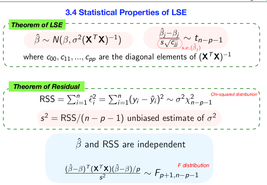
## Summary
These slides lay out the statistical assumptions required for the
Least Squares Estimator (LSE). The core idea is that if we assume the
errors are independent and normally distributed, we can then prove that:
这些幻灯片列出了最小二乘估计量 (LSE)
所需的统计假设。其核心思想是,如果我们假设误差是独立的且服从正态分布,那么我们可以证明:
Our estimated coefficients (\(\hat{\boldsymbol{\beta}}\)) also follow a
Normal distribution (or a
t-distribution when standardized). 我们的估计系数
(\(\hat{\boldsymbol{\beta}}\))
也服从正态分布(标准化后服从t
分布)。
Our summed-up squared errors (RSS) follow a Chi-squared
distribution. 我们的平方误差总和 (RSS)
服从卡方分布。
A specific ratio of the explained variance to the unexplained
variance follows an F-distribution, which is used to
test the overall significance of the model.
解释方差与未解释方差的特定比率服从F
分布,该分布用于检验模型的整体显著性。
These known distributions are the foundation for all statistical
inference in linear
models.这些已知的分布是线性模型中所有统计推断的基础。
## Deeper Dive into
Concepts and Processes
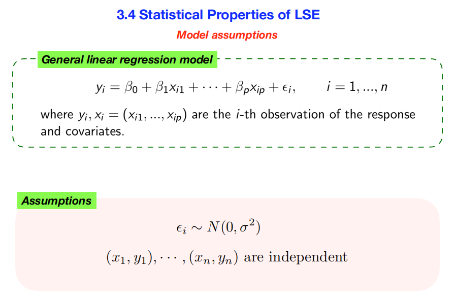
1. The Model
Assumptions (The Foundation) 模型假设(基础)
The first slide states the two assumptions that are critical for
everything that follows. Without them, we can’t make claims about the
statistical properties of our estimates.
第一张幻灯片阐述了对后续所有内容都至关重要的两个假设。没有它们,我们就无法断言估计值的统计特性。
- Assumption 1: \(\epsilon_i \sim
N(0, \sigma^2)\)
- Concept: This assumes that the error terms (the
part of
y that the model can’t explain) are drawn from a
normal (bell-curve) distribution with a mean of zero and a constant
variance \(\sigma^2\).
**假设误差项(模型无法解释的 y
值部分)服从正态(钟形曲线)分布,该分布的均值为零,方差为常数 \(\sigma^2\)。
- Meaning in Plain English:
- Mean of 0: The model is “correct on average.” The
errors are not systematically positive or negative.
**模型“平均正确”。误差并非系统地为正或负。
- Normal Distribution: Small errors are more likely
than large errors. This is a common assumption for random noise.
**小误差比大误差更有可能出现。这是随机噪声的常见假设。
- Constant Variance (\(\sigma^2\)): The amount of random
scatter around the regression line is the same at all levels of the
predictor variables. This is called homoscedasticity.
回归线周围的随机散度在预测变量的各个水平上都是相同的。这被称为同方差性。
- Assumption 2: Observations are independent
观测值是独立的**
- Concept: Each data point \((x_i, y_i)\) is an independent piece of
information. The value of the error for one observation gives no
information about the error for another observation. 每个数据点 \((x_i, y_i)\)
都是一条独立的信息。一个观测值的误差值并不能反映另一个观测值的误差。
- Meaning: This is often true for cross-sectional
data (e.g., a random sample of people) but can be violated in
time-series data where today’s error might be correlated with
yesterday’s.
这通常适用于横截面数据(例如,随机抽样的人群),但在时间序列数据中可能不成立,因为今天的误差可能与昨天的误差相关。
2.
The Distribution of the Coefficients (Theorem of LSE)
系数分布(最小二乘法定理)
This is the most important result for understanding the accuracy of
our individual predictors.
- Concept 1: The Sampling Distribution of \(\hat{\boldsymbol{\beta}}\)
Formula: \(\hat{\boldsymbol{\beta}} \sim
N(\boldsymbol{\beta},
\sigma^2(\mathbf{X}^T\mathbf{X})^{-1})\)
Meaning: If you were to take many different
random samples from the population and calculate the coefficients \(\hat{\boldsymbol{\beta}}\) for each sample,
the distribution of those coefficients would be a multivariate normal
distribution. **如果从总体中随机抽取许多不同的样本,并计算每个样本的系数
\(\hat{\boldsymbol{\beta}}\),则这些系数的分布将服从多元正态分布。
- The center of this distribution is the true population
coefficient vector \(\boldsymbol{\beta}\). This means
our estimator is unbiased—on average, it finds the
right answer. 该分布的中心是真实的总体系数向量 \(\boldsymbol{\beta}\)。这意味着我们的估计器是无偏的——平均而言,它能够找到正确的答案。
- The “spread” of this distribution is its variance-covariance matrix,
\(\sigma^2(\mathbf{X}^T\mathbf{X})^{-1}\).
This tells us the uncertainty in our estimates.
该分布的“散度”是其方差-协方差矩阵
- Concept 2: The t-statistic t 统计量
- Formula: The standardized coefficient, \(\frac{\hat{\beta}_j -
\beta_j}{\text{s.e.}(\hat{\beta}_j)}\), follows a
t-distribution with \(n-p-1\) degrees of freedom.
- Process & Meaning: In the real world, we don’t
know the true error variance \(\sigma^2\). We have to estimate it using
our sample data, which gives us \(s^2\). Because we are using an
estimate of the variance, we introduce extra uncertainty. The
t-distribution is like a normal distribution but with slightly “fatter”
tails to account for this additional uncertainty. The degrees of
freedom, \(n-p-1\), reflect the number
of data points (
n) minus the number of parameters we had to
estimate (p slopes + 1 intercept). This is the basis for
t-tests and confidence intervals for each coefficient.
在现实世界中,我们不知道真实的误差方差 \(\sigma^2\)。我们必须使用样本数据来估计它,从而得到
\(s^2\)。由于我们使用的是方差的估计值,因此引入了额外的不确定性。
t 分布类似于正态分布,但尾部略微“丰满”,以解释这种额外的不确定性。自由度
\(n-p-1\)
表示数据点的数量(n)减去我们需要估计的参数数量(p
个斜率 + 1 个截距)。这是 t 检验和每个系数置信区间的基础。
3.
The Distribution of the Error (Theorem of Residual)
误差分布(残差定理)
This theorem helps us understand the properties of our model’s
overall error.
Concept: The Residual Sum of Squares
(RSS), when scaled by the true variance, follows a
Chi-squared (\(\chi^2\))
distribution with \(n-p-1\)
degrees of freedom. 残差平方和 (RSS)
经真实方差缩放后,服从自由度为 \(n-p-1\) 的卡方 (\(\chi^2\)) 分布。
Process & Meaning: The Chi-squared
distribution often arises when dealing with sums of squared normal
variables. This theorem provides a formal probability distribution for
our total model error. Its most important consequence is that it allows
us to prove that:
**卡方分布通常用于处理正态变量的平方和。该定理为我们模型的总体误差提供了一个正式的概率分布。它最重要的推论是,它使我们能够证明:
\[s^2 = \text{RSS}/(n - p - 1)\] is
an unbiased estimate of the true error variance \(\sigma^2\). This \(s^2\) is a critical ingredient for
calculating the standard errors of our coefficients. \[s^2 = \text{RSS}/(n - p - 1)\]
是真实误差方差 \(\sigma^2\)
的无偏估计。这个 \(s^2\)
是计算系数标准误差的关键因素。
4. The
F-Distribution and the Overall Model Test
This final theorem combines our findings about the coefficients and
the residuals.
Concept: The F-statistic, which is essentially a
ratio of the variance explained by the model to the variance left
unexplained, follows an F-distribution. F
统计量本质上是模型解释的方差与未解释方差的比率,服从 F 分布。
Process & Meaning: This result relies on the
fact that our coefficient estimates (\(\hat{\boldsymbol{\beta}}\)) are independent
of our total error (RSS). The F-distribution is used for the
F-test of overall significance. This test checks the
null hypothesis that all of your slope coefficients are
simultaneously zero (\(\beta_1 = \beta_2 =
\dots = \beta_p = 0\)). If the F-test gives a small p-value, you
can conclude that your model, as a whole, is statistically significant
and provides a better fit than a model with no predictors. 如果 F
检验得出的 p
值较小,则可以得出结论,您的模型整体上具有统计显著性,并且比没有预测因子的模型拟合效果更好。
11.construct different
types of intervals
These slides explain how to use the statistical properties of the
least squares estimates to construct different types of intervals, which
are essential for quantifying the uncertainty in your model’s
predictions and parameters.
这些幻灯片解释了如何利用最小二乘估计的统计特性来构建不同类型的区间,这对于量化模型预测和参数中的不确定性至关重要。
Summary
These slides show how to calculate three distinct types of intervals
in linear regression, each answering a different question about
uncertainty:
展示了如何计算线性回归中三种不同类型的区间,每种区间分别回答了关于不确定性的不同问题:
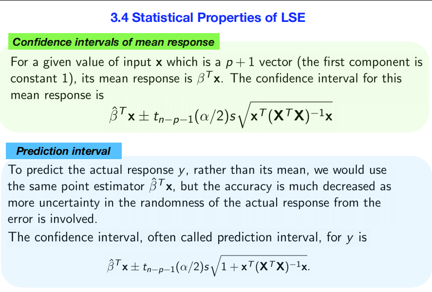
- Confidence Interval for a Parameter (\(\beta_j\)): Provides a plausible
range for a single, true unknown coefficient in the model.
为模型中单个真实未知系数提供一个合理的范围。
- Confidence Interval for the Mean Response: Provides
a plausible range for the average outcome for a given set of
predictor values.
为给定一组预测变量值的平均结果提供一个合理的范围。
- Prediction Interval: Provides a plausible range for
a single future outcome for a given set of predictor values.
This interval is always wider than the confidence interval for the mean
response because it must also account for individual random error.
为给定一组预测变量值的单个未来结果提供一个合理的范围。该区间始终比平均响应的置信区间更宽,因为它还必须考虑单个随机误差。
Deeper Dive into
Concepts and Processes
1.
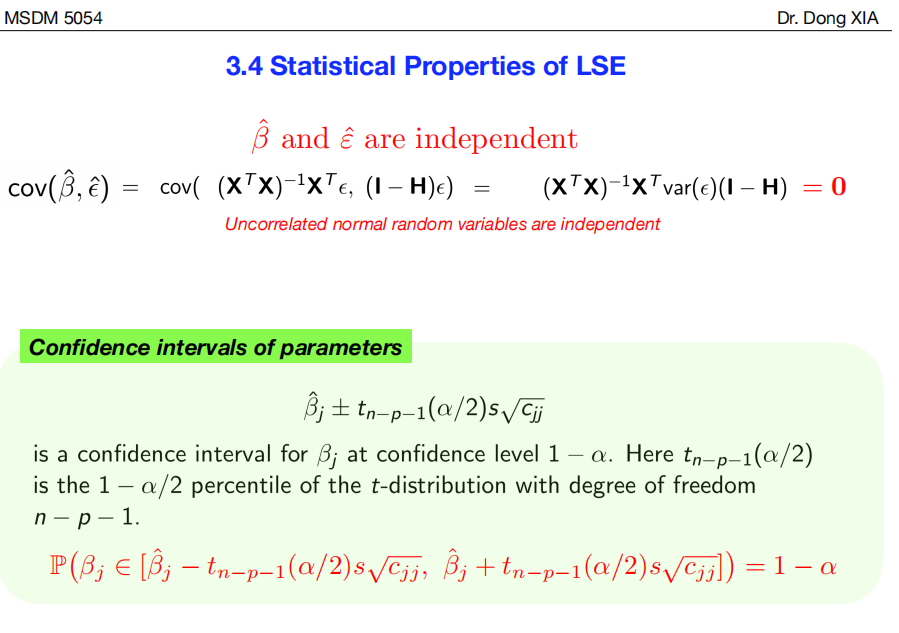
Confidence Interval for a Single Parameter 单个参数的置信区间
This interval addresses the uncertainty around one specific
coefficient, like the slope for your most important predictor.
此区间用于解决围绕某个特定系数的不确定性,例如最重要的预测因子的斜率。
- The Question It Answers: “I’ve calculated a slope
of \(\hat{\beta}_1 = 10.5\). How sure
am I about this number? What is a plausible range for the true
population slope?” 我计算出了斜率为 \(\hat{\beta}_1 =
10.5\)。我对这个数字有多确定?真实总体斜率的合理范围是多少?”
- The Formula: \(\hat{\beta}_j \pm t_{n-p-1}(\alpha/2) s
\sqrt{c_{jj}}\)
- \(\hat{\beta}_j\):
This is your best point estimate for the coefficient, taken directly
from the model output. 这是该系数的最佳点估计值,直接取自模型输出。
- \(t_{n-p-1}(\alpha/2)\): This is the
critical value from a t-distribution. It’s a multiplier
that sets the width of the interval based on your desired confidence
level (e.g., for 95% confidence, \(\alpha=0.05\)). 这是 t
分布的临界值。它是一个乘数,根据您所需的置信水平设置区间宽度(例如,对于
95% 的置信度,\(\alpha=0.05\))。
- \(s
\sqrt{c_{jj}}\): This whole term is the standard
error of the coefficient \(\hat{\beta}_j\). It measures the precision
of your estimate. A smaller standard error means a narrower, more
precise interval. 这整个项是系数 \(\hat{\beta}_j\)
的标准误差。它衡量您估计的精度。标准误差越小,区间越窄,精度越高。
2.
Confidence Interval for the Mean Response 平均响应的置信区间
This interval addresses the uncertainty about the location of the
regression line itself. 这个区间解决了回归线本身位置的不确定性。
- The Question It Answers: “For a house with 3
bedrooms and 2 bathrooms, what is the plausible range for the
average selling price of all such houses?”
它回答的问题:“对于一栋有 3 间卧室和 2
间浴室的房子,所有此类房屋的平均售价的合理范围是多少?”
- The Formula: \(\hat{\boldsymbol{\beta}}^T \mathbf{x} \pm
t_{n-p-1}(\alpha/2)s\sqrt{\mathbf{x}^T(\mathbf{X}^T\mathbf{X})^{-1}\mathbf{x}}\)
- \(\hat{\boldsymbol{\beta}}^T
\mathbf{x}\): This is your point prediction, \(\hat{y}\), for the given input vector
x. 这是给定输入向量 x 的点预测 \(\hat{y}\)。
- \(s\sqrt{\mathbf{x}^T(\mathbf{X}^T\mathbf{X})^{-1}\mathbf{x}}\):
This is the standard error of the mean response. Its value depends on
how far the input vector x is from the center of the
data. This means the confidence interval is narrowest near the average
of your data and gets wider as you move toward the extremes.
这是平均响应的标准误差。其值取决于输入向量 x
距离数据中心的距离。这意味着置信区间在数据平均值附近最窄,并且随着接近极值而变宽。
3.
Prediction Interval for an Individual Response 单个响应的预测区间
This is the most comprehensive interval and is often the most useful
for making real-world predictions.
这是最全面的区间,通常对于进行实际预测最有用。
- The Question It Answers: “I want to predict the
selling price for one specific house that has 3 bedrooms and 2
bathrooms. What is a plausible price range for this single
house?”
- The Formula: \(\hat{\boldsymbol{\beta}}^T \mathbf{x} \pm
t_{n-p-1}(\alpha/2)s\sqrt{1 +
\mathbf{x}^T(\mathbf{X}^T\mathbf{X})^{-1}\mathbf{x}}\)
- The Key Difference: Notice the formula is identical
to the one above, except for the
1 + ...
inside the square root. This “1” is critically important. It accounts
for the second source of uncertainty.
请注意,该公式与上面的公式完全相同,只是平方根中的1 + ...**不同。这个“1”至关重要。它解释了第二个不确定性来源。
- Uncertainty in the model: We are not perfectly
certain about the true location of the regression line. This is captured
by the \(\mathbf{x}^T(\mathbf{X}^T\mathbf{X})^{-1}\mathbf{x}\)
term. **我们无法完全确定回归线的真实位置。这可以通过 \(\mathbf{x}^T(\mathbf{X}^T\mathbf{X})^{-1}\mathbf{x}\)
项来捕捉。
- Uncertainty in the individual data point: Even if
we knew the true regression line perfectly, individual data points would
still be scattered around it due to random error (\(\epsilon\)). The “1” in the formula
accounts for this irreducible, random error of a single observation.
即使我们完全了解真实的回归线,由于随机误差 (\(\epsilon\)),单个数据点仍然会散布在其周围。公式中的“1”解释了单个观测值中这种不可约的随机误差。
Because it accounts for both types of uncertainty, the
prediction interval is always wider than the confidence interval
for the mean.
由于它同时考虑了两种不确定性,因此预测区间总是比均值的置信区间更宽。
The Core Difference: An
Analogy 一个类比
Confidence Interval (Mean) 均值置信区间: Like
predicting the average arrival time for a specific
flight that runs every day. After observing it for a year, you can
predict the average very accurately (e.g., 10:05 AM ± 2 minutes).
就像预测每天特定航班的平均到达时间。经过一年的观察,您可以非常准确地预测平均值(例如,上午
10:05 ± 2 分钟)。
Prediction Interval (Individual) 个体预测区间:
Like predicting the arrival time for that same flight on one
specific day next week. You have to account for the uncertainty
in the average plus the potential for random, one-time events
like weather or air traffic delays. Your prediction must be wider to be
safe (e.g., 10:05 AM ± 15 minutes).
就像预测同一航班下周某一天的到达时间。您必须考虑平均值的不确定性,以及*可能出现的随机、一次性事件,例如天气或空中交通延误。您的预测范围必须更广才能安全(例如,上午
10:05 ± 15 分钟)。
12.construct different
types of intervals
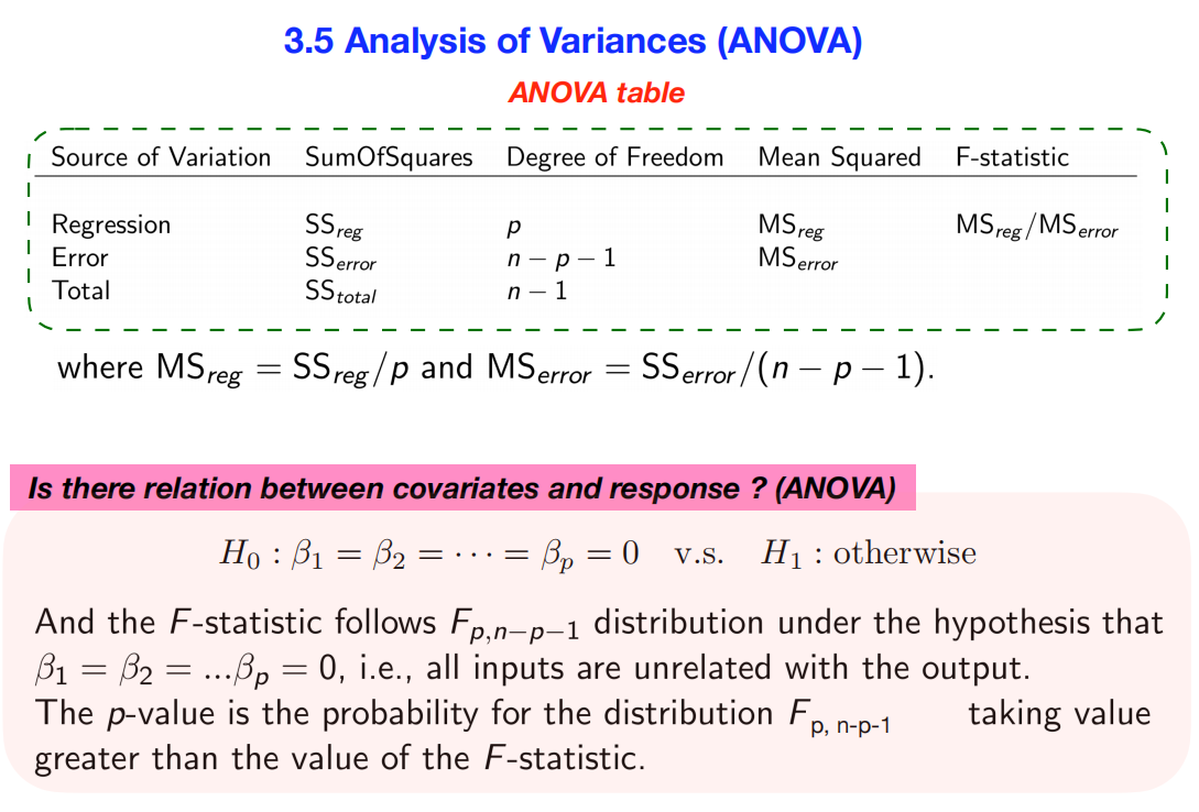
These slides explain Analysis of Variance (ANOVA), a
method used in regression to break down the total variability in your
data to test if your model is statistically significant as a
whole.这些幻灯片讲解了方差分析
(ANOVA),这是一种用于回归分析的方法,用于分解数据中的总变异性,以检验模型整体是否具有统计显著性。
Summary
The core idea is to decompose the total variation in the response
variable (Total Sum of Squares, SS_total) into two
parts: the variation that is explained by your regression model
(Regression Sum of Squares, SS_reg) and the variation
that is left unexplained (Error Sum of Squares,
SS_error).
其核心思想是将响应变量的总变异(总平方和,SS_total)分解为两部分:回归模型可以解释的变异(回归平方和,SS_reg)和未解释的变异(误差平方和,SS_error)。
By comparing the size of the explained variation to the unexplained
variation using an F-statistic, we can formally test
the hypothesis that our model has predictive power. This entire process
is neatly organized in an ANOVA table.
通过使用F
统计量比较已解释变异与未解释变异的大小,我们可以正式检验模型具有预测能力的假设。整个过程都整齐地组织在方差分析表中。
Deeper Dive into
Concepts and Connections
1.
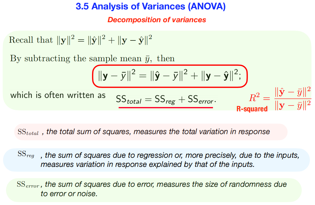
The Decomposition of Variances (The Core Equation)
方差分解(核心方程)
The first slide starts with the fundamental equation of ANOVA, which
stems directly from the geometric properties of least squares:
第一张幻灯片以方差分析的基本方程开头,该方程直接源于最小二乘的几何性质:
\[SS_{total} = SS_{reg} +
SS_{error}\]
- SS_total (Total Sum of Squares): \(\sum(y_i - \bar{y})^2\)
- Concept: This measures the total
variation in your response variable,
y. Imagine
you didn’t have a model and your only prediction for any y
was its overall average, ȳ. SS_total is the total squared
error of this simple “mean-only” model. It represents the total amount
of variation you are trying to explain.
这测量的是响应变量“y”的总变异。假设你没有模型,你对任何“y”的唯一预测是它的整体平均值“ȳ”。SS_total
是这个简单的“仅均值”模型的总平方误差。它代表了你试图解释的变异总量。
- SS_reg (Regression Sum of Squares): \(\sum(\hat{y}_i - \bar{y})^2\)
- Concept: This measures the explained
variation. It’s the amount of variation in
y that
is captured by your regression model. It calculates the difference
between your model’s predictions (ŷ) and the simple average
(ȳ). A large SS_reg means your model’s predictions are a
big improvement over just guessing the average.
它衡量解释变异**。它是回归模型捕捉到的 y
的变异量。它计算模型预测值(“ŷ”)与简单平均值(“ȳ”)之间的差异。较大的
SS_reg 意味着模型的预测结果比仅仅猜测平均值有显著改善。
- SS_error (Error Sum of Squares): \(\sum(y_i - \hat{y}_i)^2\)
- Concept: This measures the unexplained
variation (also called the Residual Sum of Squares). It’s the
amount of variation your model failed to capture. It’s the sum
of the squared differences between the actual data (
y) and
your model’s predictions (ŷ).
它衡量未解释变异**(也称为残差平方和)。它是模型未能捕捉到的变异量。它是实际数据
(y) 与模型预测值 (ŷ) 之间平方差之和。
The R-squared value is a direct consequence of this
decomposition. It’s the proportion of the total variance that is
explained by the model: R 平方
值是这种分解的直接结果。它是模型解释的总方差的比例:
\[R^2 =
\frac{SS_{reg}}{SS_{total}}\]
2. The ANOVA Table and the
F-test
方差分析表和 F 检验 The second slide organizes these sums of squares
to perform a formal hypothesis test.
第二张幻灯片整理了这些平方和,以进行正式的假设检验。
- The Question: “Is there any relationship
between my set of predictors and the response variable?” or “Is my model
better than nothing?”
“我的预测变量集和响应变量之间是否存在任何关系?”或“我的模型比没有模型好吗?”
- The Hypotheses:
- Null Hypothesis (\(H_0\)): \(\beta_1 = \beta_2 = \dots = \beta_p = 0\).
(None of the predictors have a relationship with the response; the model
is useless). 零假设 (\(H_0\)):\(\beta_1 = \beta_2 = \dots = \beta_p = 0\)。
(所有预测变量都与响应变量无关;该模型毫无用处)。
- Alternative Hypothesis (\(H_1\)): At least one \(\beta_j\) is not zero. (The model has some
predictive value). 备择假设 (\(H_1\)):至少有一个 \(\beta_j\)
不为零。(该模型具有一定的预测值)。
To test this, we can’t just compare the raw SS values, because they
depend on the number of data points and predictors. We need to normalize
them. 为了验证这一点,我们不能仅仅比较原始的 SS
值,因为它们取决于数据点和预测变量的数量。我们需要对它们进行归一化。
- Mean Squares (MS): This is the “average” variation.
We calculate it by dividing the Sum of Squares by its degrees of
freedom (df).
这是“平均”变异。我们通过将平方和除以其自由度 (df)**
来计算它。
- MS_reg = \(SS_{reg} /
p\). This is the average explained variation per
predictor. 这是每个预测变量的平均解释变异。
- MS_error = \(SS_{error} /
(n - p - 1)\). This is the average unexplained variation, which
is our estimate of the error variance, \(s^2\). 这是平均未解释变异,即我们对误差方差
\(s^2\) 的估计值。
3. The Connection:
The F-statistic 联系:F 统计量
The F-statistic is the key that connects everything.
It’s the ratio of the two mean squares: F
统计量是连接一切的关键。它是两个均方的比值: \[F = \frac{\text{Mean Squared
Regression}}{\text{Mean Squared Error}} =
\frac{MS_{reg}}{MS_{error}}\]
- Intuitive Meaning: The F-statistic is a ratio of
the average explained variation to the average
unexplained variation. F
统计量是平均解释变异与平均未解释变异的比值。
- If your model is useless (\(H_0\)
is true), the explained variation should be about the same as the
random, unexplained variation. The F-statistic will be close to 1.
如果你的模型无效(H_0$
为真),则解释变异应该与随机的未解释变异大致相同。F 统计量接近 1。
- If your model is useful (\(H_1\) is
true), the explained variation should be significantly larger than the
unexplained variation. The F-statistic will be much greater than 1.
如果你的模型有效(H_1$ 为真),则解释变异应该显著大于未解释变异。 F
统计量将远大于 1。
We compare our calculated F-statistic to an
F-distribution to get a p-value. A
small p-value (< 0.05) provides strong evidence to reject the null
hypothesis and conclude that your model, as a whole, is statistically
significant. 我们将计算出的 F 统计量与F
分布进行比较,得出p 值。较小的 p 值(<
0.05)可以提供强有力的证据来拒绝零假设,并得出您的模型整体具有统计显著性的结论。
12.construct different
types of intervals
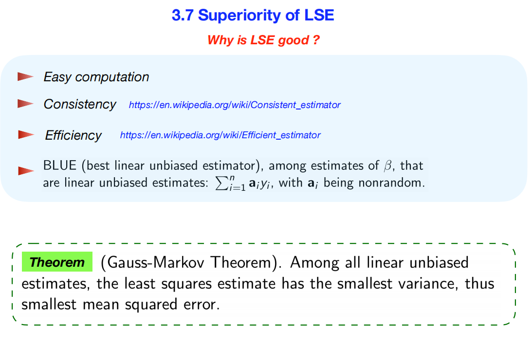
- 内容: These slides explain the Gauss-Markov
theorem, a cornerstone result in statistics that establishes
why the Least Squares Estimator (LSE) is considered the gold standard
for fitting linear models under a specific set of assumptions.
这些幻灯片解释了高斯-马尔可夫定理,这是统计学中的一个基石性成果,它阐明了为什么最小二乘估计量
(LSE) 被认为是在特定假设条件下拟合线性模型的黄金标准。
Summary
The slides argue for the superiority of the Least Squares Estimator
(LSE) by highlighting its key properties: it’s easy to compute,
consistent, and efficient. This culminates in the Gauss-Markov
Theorem, which proves that LSE is BLUE: the
Best Linear Unbiased
Estimator. This means that among all estimators that
are both linear and unbiased, the LSE is the “best” because it has the
smallest possible variance, making it the most precise. The second slide
provides the key steps for the mathematical proof of this important
theorem. 这些幻灯片通过强调最小二乘估计量 (LSE)
的关键特性来论证其优越性:易于计算、一致性高且高效。最终得出了高斯-马尔可夫定理,该定理证明了
LSE
是BLUE:最佳线性无偏估计量。这意味着在所有线性且无偏的估计量中,LSE
是“最佳”的,因为它具有最小的方差,因此精度最高。第二张幻灯片提供了这一重要定理的数学证明的关键步骤。
Deeper Dive into the
Concepts
Properties of
LSE (Slide 1) 局部正交估计 (LSE) 的性质
- Easy Computation易于计算: The LSE has a direct,
closed-form solution called the Normal Equation (\(\hat{\boldsymbol{\beta}} =
(\mathbf{X}^T\mathbf{X})^{-1}\mathbf{X}^T\mathbf{y}\)). You can
calculate it directly without needing complex iterative algorithms.
- Consistency一致性: As your sample size gets larger
and larger, the LSE estimate (\(\hat{\boldsymbol{\beta}}\)) is guaranteed
to get closer and closer to the true population value (\(\boldsymbol{\beta}\)). With enough data, it
will find the truth. 随着样本量越来越大,LSE 估计值 (\(\hat{\boldsymbol{\beta}}\))
必然会越来越接近真实的总体值 (\(\boldsymbol{\beta}\))。只要有足够的数据,它就能找到真相。
- Efficiency效率: An efficient estimator is the one
with the lowest possible variance. This means its estimates are the most
precise and least spread out.
高效的估计器是方差尽可能低的估计器。这意味着它的估计值最精确,且分布最均匀。
- BLUE (Best Linear Unbiased
Estimator)BLUE(最佳线性无偏估计器): This acronym elegantly
summarizes the Gauss-Markov theorem.
这个缩写完美地概括了高斯-马尔可夫定理。
- Linear: The estimator is a linear function of the
response variable y. We can write it as \(\hat{\boldsymbol{\beta}} =
\mathbf{A}\mathbf{y}\) for some matrix A.
估计器是响应变量y的线性函数。对于某个矩阵A,我们可以将其写成
\(\hat{\boldsymbol{\beta}} =
\mathbf{A}\mathbf{y}\)。
- Unbiased: The estimator does not systematically
overestimate or underestimate the true parameter. On average, its
expected value is the true value: \(E[\hat{\boldsymbol{\beta}}] =
\boldsymbol{\beta}\).
估计器不会系统性地高估或低估真实参数。平均而言,其预期值即为真实值:\(E[\hat{\boldsymbol{\beta}}] =
\boldsymbol{\beta}\)。
- Best: It has the minimum variance
of all possible linear unbiased estimators. It’s the most precise and
reliable estimator in its class.
在所有可能的线性无偏估计器中,它的方差最小。它是同类中最精确、最可靠的估计器。
The Gauss-Markov
Theorem 高斯-马尔可夫定理
The theorem provides the theoretical justification for using OLS.
该定理为使用最小二乘法 (OLS) 提供了理论依据。 * The Core
Idea: You could invent many different ways to estimate the
coefficients of a linear model. As long as your proposed methods are
both linear and unbiased, the Gauss-Markov theorem guarantees that none
of them will be more precise than the standard least squares method. LSE
gives the “sharpest” possible estimates.
你可以发明许多不同的方法来估计线性模型的系数。只要你提出的方法是线性的且无偏的,高斯-马尔可夫定理就能保证,它们都不会比标准最小二乘法更精确。最小二乘法
(LSE) 给出了“最精确”的估计值。
- The Logic of the Proof (Slide 2) 证明逻辑: The
proof is a clever comparison of variances. **该证明巧妙地比较了方差。
- It starts by defining any other linear unbiased
estimator as \(\tilde{\boldsymbol{\beta}} =
\mathbf{A}\mathbf{y}\).
首先,将任何其他线性无偏估计量定义为 \(\tilde{\boldsymbol{\beta}} =
\mathbf{A}\mathbf{y}\)。
- It uses the “unbiased” property to force a condition on the matrix
A, which ultimately leads to the insight that
A can be written in terms of the LSE matrix plus some
other matrix D, where DX = 0.
它利用“无偏”性质对矩阵A强制施加一个条件,最终得出A可以写成LSE矩阵加上另一个矩阵D,其中DX
= 0。
- It then calculates the variance of this other estimator, which turns
out to be: \[Var(\tilde{\boldsymbol{\beta}})
= Var(\text{LSE}) + \text{a non-negative term involving }
\mathbf{D}\] 然后计算另一个估计量的方差,结果为: \[Var(\tilde{\boldsymbol{\beta}}) = Var(\text{LSE})
+ \text{一个包含 } \mathbf{D} 的非负项\]
- Since the variance of any other linear unbiased estimator is the
variance of the LSE plus something non-negative, the variance
of the LSE must be the smallest possible value.
由于任何其他线性无偏估计量的方差都是LSE的方差加上一个非负项,因此LSE的方差必须是最小的可能值。
Further Understandings
Beyond the Slides
1. What are the
required assumptions?需要哪些假设?
The Gauss-Markov theorem is powerful, but it’s not magic. It only
holds if a set of assumptions about the model’s errors (\(\epsilon\)) are met:
高斯-马尔可夫定理虽然强大,但并非魔法。它仅在满足以下关于模型误差 (\(\epsilon\)) 的假设时成立: * Zero
Mean零均值: The average of the errors is zero (\(E[\epsilon] = 0\)). 误差的平均值为零 (\(E[\epsilon] = 0\))。 * Constant
Variance (Homoscedasticity)恒定方差(同方差性): The errors
have the same variance, \(\sigma^2\),
at all levels of the predictors.
在预测变量的各个水平上,误差具有相同的方差 \(\sigma^2\)。 * Uncorrelated
Errors不相关误差:** The error for one observation is not correlated with
the error for another. 一个观测值的误差与另一个观测值的误差不相关。 *
No Perfect Multicollinearity非完全多重共线性: The
predictor variables are not perfectly linearly related.
预测变量并非完全线性相关。
Crucially, the Gauss-Markov theorem does NOT require the
errors to be normally distributed. The normality assumption is
only needed later for constructing confidence intervals and conducting
t-tests and F-tests.
至关重要的是,高斯-马尔可夫定理并不要求误差服从正态分布。**正态性假设仅在构建置信区间以及进行
t 检验和 F 检验时需要。
2.
When is LSE NOT the Best? (The Bias-Variance Tradeoff) 什么时候 LSE
不是最佳选择? (偏差-方差权衡)
While LSE is the best unbiased estimator, sometimes we can
get better predictive performance by accepting a little bit of bias in
exchange for a large reduction in variance. This is the core idea behind
modern regularization methods: 虽然 LSE
是最好的无偏估计器,但有时我们可以通过接受少量偏差来大幅降低方差,从而获得更好的预测性能。这是现代正则化方法背后的核心思想:
* Ridge Regression and LASSO岭回归和 LASSO: These are
popular techniques that produce biased estimates of the
coefficients. However, by introducing this small amount of bias, they
can often produce models with a lower overall error (Mean Squared Error)
than LSE, especially when predictors are highly correlated.
这些是产生有偏系数估计的流行技术。然而,通过引入少量偏差,它们通常可以生成比
LSE
具有更低总体误差(均方误差)的模型,尤其是在预测变量高度相关的情况下。
Therefore, while LSE is the theoretical champion in the world of
unbiased estimators, in the world of predictive modeling, methods that
intentionally introduce bias can sometimes be superior. 因此,虽然 LSE
是无偏估计领域的理论冠军,但在预测模型领域,有意引入偏差的方法有时会更胜一筹。