PHYS 5120 - Computational Energy Materials and Electronic Structure Simulations-W10-1

PHYS 5120 - 计算能源材料和电子结构模拟 Lecture

Lecturer: Prof.PAN DING

Based on the whiteboard image, these notes cover advanced topics in Density Functional Theory (DFT), specifically focusing on two major challenges: the treatment of Van der Waals (dispersion) forces and the physical interpretation of Kohn-Sham (KS) eigenstates (specifically the bandgap problem).

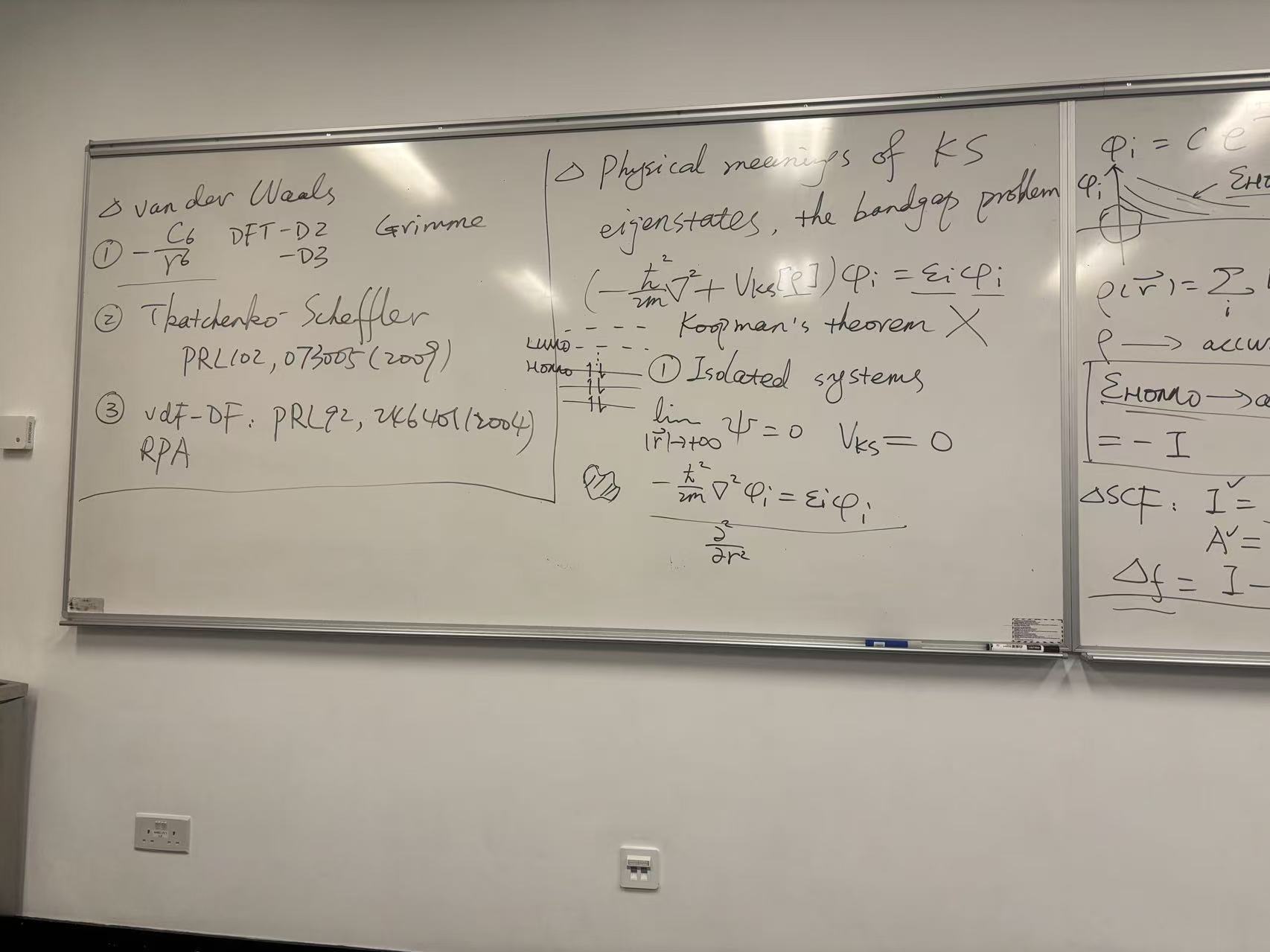
1. Left Panel: Van der Waals (vdW) Corrections

Standard DFT functionals (like LDA or GGA) often fail to describe long-range dispersion interactions (Van der Waals forces). The board lists three common strategies to correct this:

• Method 1: Semi-empirical Corrections (Grimme methods)
  • Notation: \(-\frac{C_6}{r^6}\)
  • Keywords: DFT-D2, DFT-D3, Grimme.
  • Explanation: This approach adds a simple pairwise semi-empirical potential term (based on the \(1/r^6\) decay) to the total energy to account for dispersion.
• Method 2: Tkatchenko-Scheffler (TS)
  • Citation: PRL 102, 073005 (2009)
  • Explanation: This refers to a method that derives dispersion coefficients (\(C_6\)) from the electron density itself, making it less empirical than standard Grimme corrections.
• Method 3: vdW-DF (Van der Waals Density Functional)
  • Citation: PRL 92, 246401 (2004)
  • Explanation: This refers to the Dion et al. functional, which includes a non-local correlation term to physically describe dispersion without empirical parameters.
• RPA (Random Phase Approximation): Listed at the bottom, this is a more computationally expensive method that naturally accounts for non-local electron correlation (including vdW) from first principles.

2. Middle Panel: KS Eigenstates & The Bandgap Problem

This section discusses the physical meaning of the eigenvalues obtained from the Kohn-Sham equations.

• The Kohn-Sham Equation: The board displays the fundamental equation for a single particle in an effective potential: \[\left(-\frac{\hbar^2}{2m}\nabla^2 + V_{KS}[\rho]\right) \phi_i = \epsilon_i \phi_i\]

• The “Bandgap Problem”:

  • Context: The notes mention “Koopmans’ theorem X”. In Hartree-Fock theory, Koopmans’ theorem links orbital energies to ionization energies. In DFT, this relationship is not straightforward for all orbitals.
  • The Issue: Standard DFT functionals typically underestimate the bandgap (the energy difference between the occupied and unoccupied states).

• Isolated Systems Limit: The notes explore the behavior of the wavefunction at the boundary:

  • Limit: \(\lim_{|\vec{r}|\to\infty} \psi = 0\) and \(V_{KS} = 0\)
  • Asymptotic behavior: \[-\frac{\hbar^2}{2m} \nabla^2 \phi_i = \epsilon_i \phi_i\] This describes the decay of the wavefunction far from the nucleus.

3. Right Panel (Partially Visible)

This section connects the Highest Occupied Molecular Orbital (HOMO) to physical observables.

• Asymptotic Decay: \(\phi_i = C e^{-\kappa r}\) (implied by the math). The decay rate of the density depends on the ionization potential.
• The Exact Condition: The text \(\epsilon_{HOMO} \to -I\) indicates a fundamental theorem in exact DFT: The energy of the highest occupied Kohn-Sham orbital is exactly equal to the negative of the ionization potential (\(I\)).
• \(\Delta\)SCF: This refers to the “Delta Self-Consistent Field” method, a way to calculate ionization energies or excitation energies by explicitly calculating the energy difference between the neutral and charged species (\(E_{N-1} - E_N\)), rather than relying solely on orbital eigenvalues.

Summary of References Cited

If you need to look up the specific papers mentioned on the left side of the board, here they are:

1. Tkatchenko & Scheffler: Phys. Rev. Lett. 102, 073005 (2009). “Accurate Molecular Van Der Waals Interactions from Ground-State Electron Density and Free-Atom Reference Data.”

2. Dion et al. (vdW-DF): Phys. Rev. Lett. 92, 246401 (2004). “Van der Waals Density Functional for General Geometries.”

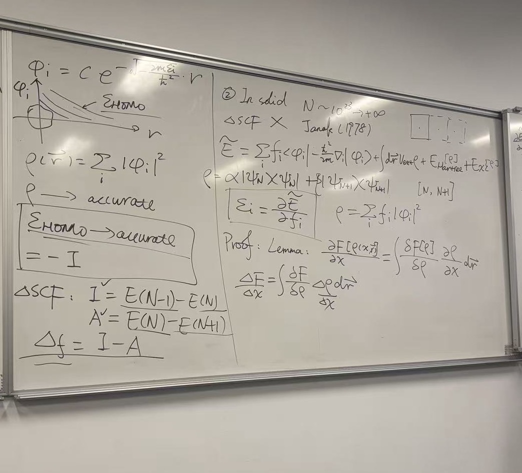
This image provides a deeper dive into the physical interpretation of Kohn-Sham eigenvalues, specifically contrasting how we treat finite systems (like molecules) versus infinite solids, and introducing the fundamental Janak’s Theorem.

Here is the breakdown of the notes, moving from left to right.

1. Left Panel: Finite Systems & The Meaning of \(\epsilon_{HOMO}\)

This section focuses on isolated systems (atoms/molecules) where the wavefunction decays to zero at infinity.

• Asymptotic Decay: The notes show the wavefunction \(\phi_i\) decaying exponentially as \(r \to \infty\): \[\phi_i \propto e^{-\sqrt{\frac{2m|\epsilon_i|}{\hbar^2}} r}\] This decay rate is determined physically by the Ionization Potential (\(I\)).

• The Exact DFT Condition: The box highlights a crucial theorem in exact DFT: \[\epsilon_{HOMO} = -I\] The eigenvalue of the Highest Occupied Molecular Orbital (HOMO) is physically meaningful—it equals the negative of the Ionization Potential. (Note: This is strictly true only for the exact functional, though approximate functionals often get the density right but the energy wrong).

• \(\Delta\)SCF Method: Since eigenvalues (\(\epsilon\)) in approximate DFT are often inaccurate, we use the Delta Self-Consistent Field (\(\Delta\)SCF) method to calculate gaps explicitly:

  • Ionization Potential (\(I'\)): \(E(N-1) - E(N)\)
  • Electron Affinity (\(A'\)): \(E(N) - E(N+1)\)
  • Fundamental Gap (\(\Delta_f\)): \(I - A\) This involves doing three separate calculations (neutral, cation, anion).

2. Right Panel: Solids & Janak’s Theorem

This is the most technically significant part of the board. It addresses the problem: How do we define these energies in a bulk solid where removing one electron from \(10^{23}\) atoms is negligible?

• The Problem with Solids: The notes state: In solid N ~ 10^23 -> infinity. It immediately notes Delta SCF X, meaning the \(\Delta\)SCF method is not practical or well-defined for calculating bandgaps in infinite periodic solids.

• Janak’s Theorem (1978):

  • Citation: Janak, Phys. Rev. B 18, 7165 (1978).
  • Concept: Janak generalized DFT to allow for fractional occupation numbers (\(f_i\)), where \(0 \le f_i \le 1\).
  • The Boxed Equation: \[\epsilon_i = \frac{\partial \tilde{E}}{\partial f_i}\] This is Janak’s Theorem. It states that the Kohn-Sham orbital energy \(\epsilon_i\) is the derivative of the total energy with respect to the occupation number of that orbital.

• Implication: This theorem connects the mathematical Lagrange multipliers (the eigenvalues \(\epsilon_i\)) to a physical derivative. It is the foundation for understanding why the “Bandgap Problem” exists.

  • In exact DFT, the energy \(E\) as a function of fractional electron number should be a series of straight lines (linearity condition).
  • Because standard functionals (LDA/GGA) are not linear (they are convex), the derivative \(\frac{\partial E}{\partial f_i}\) is incorrect at integer points, leading to the wrong bandgap.

• The Lemma/Proof (Bottom Right): The notes sketch the proof using the chain rule for functional derivatives: \[\frac{\partial F[\rho]}{\partial x} = \int \frac{\delta F[\rho]}{\delta \rho} \frac{\partial \rho}{\partial x} d\vec{r}\] This mathematical machinery is used to prove that the variation in energy comes from the variation in density caused by changing the occupation \(f_i\).

Summary of the Lesson

The board is teaching the derivation of the bandgap: 1. For Molecules: We can use \(\Delta\)SCF (calculating \(N\) and \(N \pm 1\) systems) to find the exact gap. 2. For Solids: We cannot use \(\Delta\)SCF. We must rely on the eigenvalues \(\epsilon_i\). 3. Janak’s Theorem proves that \(\epsilon_i\) is the derivative of the energy. 4. Therefore, if our energy functional has the wrong curvature (derivative) with respect to electron count (which LDA/GGA do), our bandgaps in solids will inevitably be wrong.

This concept is the “Holy Grail” for understanding why standard DFT fails to predict bandgaps correctly. It connects the math on the right side of your whiteboard (Janak’s Theorem) to the physical reality of electrons.

The explanation of Derivative Discontinuity and the Straight Line Condition.

1. The “Straight Line” Graph (Exact DFT)

Imagine a graph where the X-axis is the number of electrons (\(N\)) in a system, and the Y-axis is the Total Energy (\(E\)).

In the real world (and in exact DFT), electrons are discrete. You can have 1 electron or 2, but you cannot have 1.5 electrons on a single atom unless you treat it as a statistical ensemble (50% probability of having 1, 50% probability of having 2).

If you plot the energy for fractional electrons in exact DFT, the graph consists of straight line segments connecting the integer points.

• Slope to the left of integer \(N\): The energy cost to remove an electron. By definition, this slope is \(-I\) (Ionization Potential).
• Slope to the right of integer \(N\): The energy cost to add an electron. By definition, this slope is \(-A\) (Electron Affinity).

2. The “Discontinuity”

Here is the critical part: The slope changes abruptly at the integer.

The energy cost to remove an electron from a stable shell is high. The energy gain from adding an electron to a new, higher energy shell is low. Therefore, the slope on the left is steep, and the slope on the right is shallow.

• Janak’s Theorem (from your board) says: \(\epsilon = \frac{\partial E}{\partial f}\) (The eigenvalue is the slope).
• Because the slope changes, the eigenvalue \(\epsilon\) should jump as you cross the integer \(N\).
• This jump is called the Derivative Discontinuity (\(\Delta_{xc}\)).

The true fundamental gap (\(E_{gap}\)) is the difference between these two slopes: \[E_{gap} = I - A\]

3. The Problem with LDA/GGA (The “Convex” Curve)

Standard functionals like LDA or GGA violate this straight-line condition. Instead of a straight line, they produce a convex curve (like a hanging chain or a U-shape) between integers.

Because the curve is smooth and convex: 1. There is no jump in the slope at the integer \(N\). The slope just before \(N\) is almost the same as the slope just after \(N\). 2. This means the energy of the highest occupied state (\(\epsilon_{HOMO}\)) is predicted to be too high (too unstable), and the lowest unoccupied state (\(\epsilon_{LUMO}\)) is too low. 3. Result: The calculated bandgap is significantly smaller than the real bandgap.

4. Summary: The Equation

This leads to the famous decomposition of the bandgap.

In exact DFT, the true fundamental gap (\(E_{gap}\)) is the sum of the Kohn-Sham orbital gap (\(\epsilon_{gap}^{KS}\)) plus the discontinuity constant (\(\Delta_{xc}\)):

\[E_{gap} = \underbrace{(\epsilon_{LUMO} - \epsilon_{HOMO})}_{\text{DFT Bandgap}} + \underbrace{\Delta_{xc}}_{\text{Derivative Discontinuity}}\]

• In Exact DFT: \(\Delta_{xc}\) is large and positive. It accounts for the jump.
• In LDA/GGA: \(\Delta_{xc}\) is wrongly zero (or very close to it).
• Therefore: \(E_{gap} \approx \epsilon_{gap}^{KS}\). Since we are missing the positive \(\Delta_{xc}\) term, the DFT bandgap is underestimated (often by 30-50%).

How this connects to your whiteboard

On the right panel, the notes mention “In solid… \(\Delta\)SCF X”.

• For a molecule, you can manually calculate \(E(N)\) and \(E(N+1)\) to find the slopes (the \(\Delta\)SCF method).
• For a solid, you can’t easily add 1 electron to a bulk crystal. You have to rely on the eigenvalues (\(\epsilon\)).
• Since standard DFT (LDA/GGA) misses the Derivative Discontinuity, the eigenvalues \(\epsilon\) don’t reflect the true energy cost of adding/removing electrons, leading to the bandgap problem.

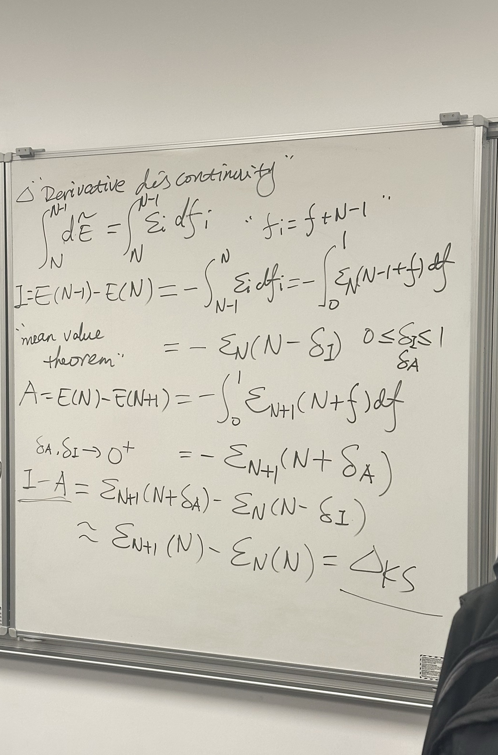
The mathematical proof of the “Derivative Discontinuity” concept we just discussed. It uses calculus to derive exactly why the standard DFT bandgap (\(\Delta_{KS}\)) is often an approximation that misses the real physics.

Here is the step-by-step breakdown of the derivation on the board:

1. Top Section: From Janak’s Theorem to Energy Differences

The derivation starts with Janak’s Theorem (\(\epsilon_i = \partial E / \partial f_i\)). To find the total energy difference between integer electron counts (like \(N\) and \(N-1\)), we must integrate this derivative.

• Equation: \(\int_N^{N-1} d\tilde{E} = \int_N^{N-1} \epsilon_i df_i\)
• Translation: The energy change when removing an electron is the sum (integral) of the orbital energy values as you slowly drain the electron density from \(1.0\) down to \(0.0\).

2. Middle Section: Defining Ionization (\(I\)) and Affinity (\(A\))

The board uses the Mean Value Theorem for integrals. This theorem states that \(\int_a^b g(x)dx = (b-a)g(c)\) for some point \(c\) in the interval.

• For Ionization Potential (\(I\)): \[I = E(N-1) - E(N)\] Using the Mean Value Theorem, this integral is equal to the eigenvalue \(\epsilon_N\) evaluated at some fractional electron count \(N - \delta_I\) (where \(0 \le \delta_I \le 1\)). \[I = -\epsilon_N(N-\delta_I)\]

• For Electron Affinity (\(A\)): \[A = E(N) - E(N+1)\] Similarly, this equals the eigenvalue of the next orbital (\(\epsilon_{N+1}\)) evaluated at a fractional count \(N+\delta_A\). \[A = -\epsilon_{N+1}(N+\delta_A)\]

3. Bottom Section: The Gap and the Approximation

This is the most important part. It combines \(I\) and \(A\) to find the Fundamental Gap (\(I - A\)).

• The Exact Gap: \[I - A = \epsilon_{N+1}(N+\delta_A) - \epsilon_N(N-\delta_I)\] This equation says the true gap depends on the eigenvalues at fractional occupations slightly away from the neutral state.

• The Approximation (The “Kohn-Sham Gap”): The last line shows what happens in standard DFT (LDA/GGA): \[\approx \epsilon_{N+1}(N) - \epsilon_N(N) = \Delta_{KS}\]

  Why is this an approximation? This step assumes that the eigenvalues \(\epsilon\) do not change significantly as you change the occupation numbers (\(\delta \to 0\)).

  • If there is no derivative discontinuity (like in LDA/GGA), the eigenvalues are continuous, so \(\epsilon(N+\delta) \approx \epsilon(N)\).
  • Therefore, you get the standard result: The Gap = LUMO energy - HOMO energy.

This board proves that \(\Delta_{KS}\) (the orbital gap) is only equal to the Fundamental Gap (\(I-A\)) if the derivative discontinuity is zero.

Since we know from exact quantum mechanics that the discontinuity is NOT zero (the slope must jump at integers), this derivation proves mathematically why standard DFT functionals (which lack this jump) are theoretically guaranteed to underestimate the bandgap.

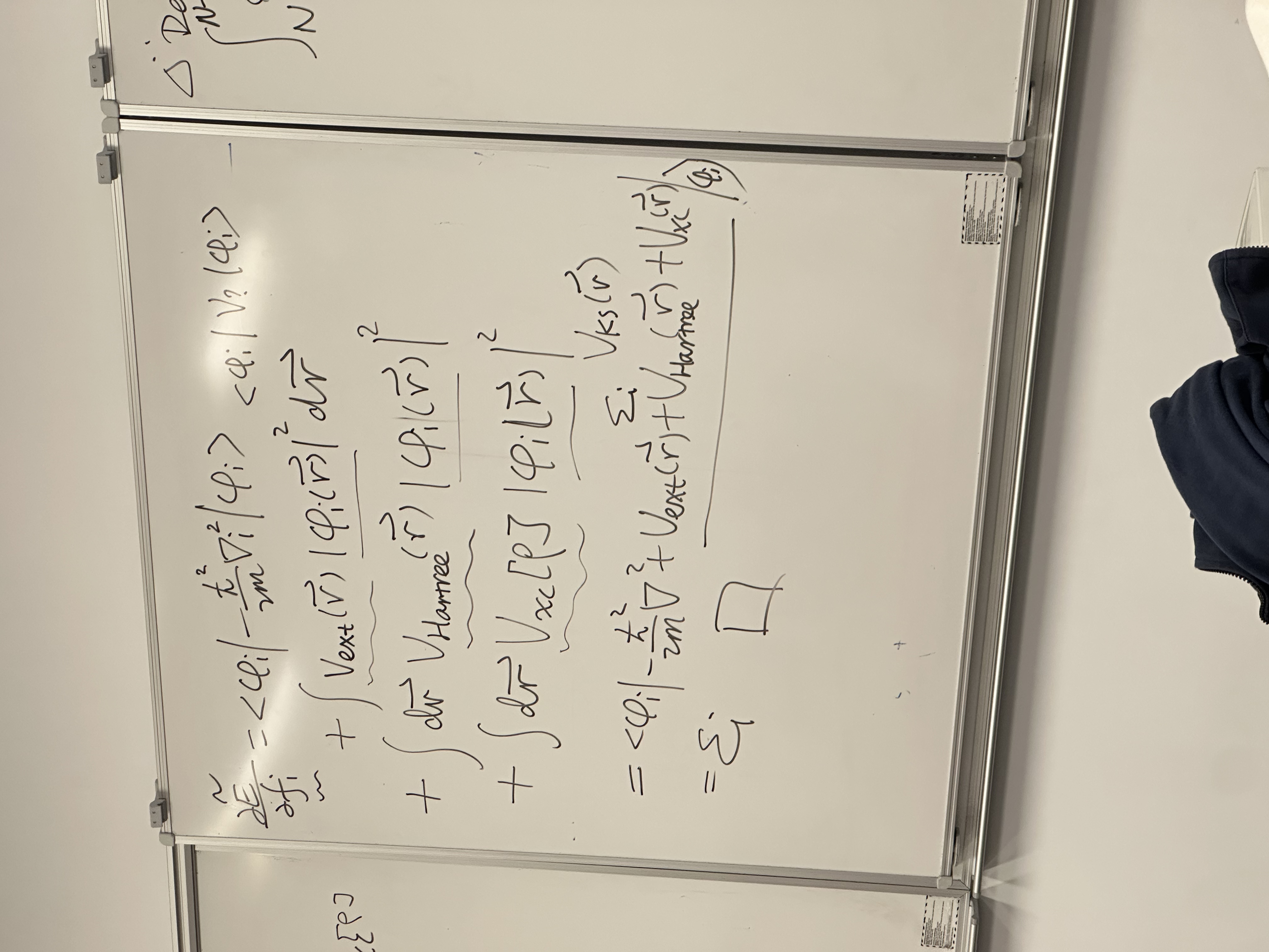
This whiteboard contains the detailed mathematical derivation (proof) of Janak’s Theorem, which was introduced on the previous board.

Recall the theorem’s statement: \(\frac{\partial E}{\partial f_i} = \epsilon_i\). (The derivative of the total energy with respect to the occupation number of an orbital is equal to that orbital’s eigenvalue).

Here is the line-by-line breakdown of the proof shown on the board:

1. The Goal

The derivation starts at the top left: \[\frac{\partial \tilde{E}}{\partial f_i} = \dots\] We are calculating how the total energy changes when we add a tiny fraction of an electron to orbital \(i\).

2. Term-by-Term Differentiation

The total energy in DFT is a sum of Kinetic, External, Hartree, and Exchange-Correlation energies. The derivation differentiates each part separately:

• Kinetic Energy Term (Top Line): \[\langle \phi_i | -\frac{\hbar^2}{2m} \nabla^2 | \phi_i \rangle\] This is the expectation value of the kinetic energy for orbital \(i\).

• External Potential Term (2nd Line): \[+ \int V_{ext}(\vec{r}) |\phi_i(\vec{r})|^2 d\vec{r}\] Since the density \(\rho = \sum f_i |\phi_i|^2\), the derivative \(\frac{\partial \rho}{\partial f_i}\) is simply \(|\phi_i|^2\). This term represents the interaction of the specific orbital \(i\) with the nuclei.

• Hartree Term (3rd Line): \[+ \int d\vec{r} V_{Hartree}(\vec{r}) |\phi_i(\vec{r})|^2\] The derivative of the total Hartree energy with respect to density gives the Hartree Potential (\(V_{Hartree}\)).

• Exchange-Correlation Term (4th Line): \[+ \int d\vec{r} V_{xc}[\rho] |\phi_i(\vec{r})|^2\] Similarly, the derivative of the XC energy gives the XC Potential (\(V_{xc}\)).

3. Recombining the Terms

The lecturer then groups all these terms together into a single expectation value bracket:

\[= \langle \phi_i | -\frac{\hbar^2}{2m} \nabla^2 + \underbrace{V_{ext}(\vec{r}) + V_{Hartree}(\vec{r}) + V_{xc}(\vec{r})}_{V_{KS}(\vec{r})} | \phi_i \rangle\]

• The sum of the three potentials (External + Hartree + XC) is exactly the definition of the Kohn-Sham Effective Potential (\(V_{KS}\)).
• Therefore, the operator inside the bracket is the Kohn-Sham Hamiltonian (\(H_{KS}\)).

4. The Conclusion (Q.E.D.)

The final step relies on the Kohn-Sham equation itself (\(H_{KS} \phi_i = \epsilon_i \phi_i\)):

\[= \epsilon_i \quad \square\]

The expectation value of the Hamiltonian for an eigenvector is simply the eigenvalue. The square box (\(\square\)) is the symbol for “Q.E.D.” (quod erat demonstrandum), indicating the proof is complete.

Why this matters in the context of the lecture?

This proof solidifies the previous discussion about the bandgap. It mathematically proves that the eigenvalue \(\epsilon_i\) really is the energy cost of adding a fractional electron.

If the functional (like LDA/GGA) gets the energy curvature wrong (no derivative discontinuity), this derivative \(\epsilon_i\) will yield the wrong value for the gap, as shown in the previous slides.

This final whiteboard image brings the entire derivation to its “grand conclusion.” It combines the definitions of Ionization Potential (\(I\)) and Electron Affinity (\(A\)) to show exactly why standard DFT gets the bandgap wrong and what the missing piece is.

Here is the breakdown of the derivation on the board:

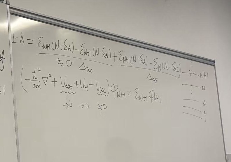
1. The “Magic” Decomposition (Top Equation)

The lecturer takes the definition of the fundamental gap (\(I - A\)) derived in the previous slide and performs a clever algebraic split by adding and subtracting the term \(\epsilon_{N+1}(N-\delta)\) (essentially the LUMO energy of the neutral system).

\[I - A = \underbrace{\epsilon_{N+1}(N+\delta_A) - \epsilon_{N+1}(N-\delta_A)}_{\Delta_{xc}} + \underbrace{\epsilon_{N+1}(N-\delta_A) - \epsilon_{N}(N-\delta_I)}_{\Delta_{KS}}\]

This splits the true bandgap into two distinct physical components:

• \(\Delta_{KS}\) (The Kohn-Sham Gap): This is the standard gap you get from a DFT output: LUMO energy minus HOMO energy.
  • \(\Delta_{KS} = \epsilon_{N+1}(N) - \epsilon_{N}(N)\)
• \(\Delta_{xc}\) (The Derivative Discontinuity): This is the “missing piece.” It represents how much the eigenvalue \(\epsilon_{N+1}\) jumps when you cross the integer electron count \(N\).
  • Mathematically: \(\lim_{\delta \to 0} [\epsilon_{N+1}(N+\delta) - \epsilon_{N+1}(N-\delta)]\)
  • The board notes: \(\neq 0\) (This term is not zero in exact theory).

2. The “Culprit” in the Hamiltonian (Middle Equation)

The board asks: Where does this discontinuity come from?

It writes out the Kohn-Sham equation for the \((N+1)\)-th electron: \[\left(-\frac{\hbar^2}{2m}\nabla^2 + V_{ext} + V_H + V_{xc}\right) \phi_{N+1} = \epsilon_{N+1} \phi_{N+1}\]

Underneath the potential terms, there are small arrows indicating whether these potentials experience a “jump” (discontinuity) when the electron count changes infinitesimally:

• \(V_{ext}\) (External Potential): \(\to 0\). The nuclear potential is fixed; it doesn’t care about electron count. It is continuous.
• \(V_{H}\) (Hartree Potential): \(\to 0\). The classical electrostatic potential is continuous with respect to small density changes.
• \(V_{xc}\) (Exchange-Correlation Potential): \(\neq 0\).
  • This is the key insight: The Exchange-Correlation potential jumps by a constant constant value everywhere in space the moment you add a fraction of an electron past integer \(N\).

3. The Final Conclusion

The fundamental gap is the sum of the calculated gap and this potential jump:

\[E_{gap}^{fund} = \Delta_{KS} + \Delta_{xc}\]

• In Standard DFT (LDA/GGA): The functional is smooth. It has no derivative discontinuity (\(\Delta_{xc} \approx 0\)). Therefore, \(E_{gap} \approx \Delta_{KS}\). This is why standard DFT underestimates the bandgap—it is missing the \(\Delta_{xc}\) term entirely.
• In Exact DFT: The potential \(V_{xc}\) jumps, providing the necessary energy correction to match the experimental gap (\(I-A\)).

Summary of the Full Lecture Sequence

Based on your four images, here is the complete narrative of the lecture:

1. The Problem: Standard DFT fails at Van der Waals forces and Bandgaps.
2. The Tool: Janak’s Theorem connects eigenvalues (\(\epsilon\)) to the derivative of energy (\(\partial E / \partial f\)).
3. The Proof: Using calculus, we proved Janak’s theorem and showed that the true gap depends on the slopes of the energy curve.
4. The Verdict (This Slide): The true gap (\(I-A\)) equals the DFT orbital gap (\(\Delta_{KS}\)) PLUS a derivative discontinuity (\(\Delta_{xc}\)). Standard functionals miss this discontinuity, which is why they fail for solids/semiconductors.